Unkneading
It’s time to explore the inner workings of deep neural nets in more detail.
Consider a perceptron trained to recognize bananas on sight, in all their variations and orientations, against any background. Normally this would involve a final one-hot layer in the neural net containing a “banana neuron”; since we need at least two neurons for such an output layer, let’s also assume a “not-banana neuron” lights up in response to everything else. Supervised training of this model would involve curating many images of either bananas or something else, each labeled with a single bit specifying which of the two neurons should activate. By the end of the training, we’d have a banana detector. 1
Recall from chapter 3 that in a convolutional net, higher-order features emerge hierarchically as combinations of lower-level features. As activations propagate to higher layers in the network, the features represented become increasingly invariant—that is, more semantically meaningful.
I think of the process as a bit like kneading dough. Every layer of a neural net works its input data, turning it like a ball of dough in a certain direction and then pressing it down, flattening it as if against a countertop. Then the next layer does the same. Understanding how and why this “data kneading” accomplishes anything will require deeper insight into how the successive layers of a neural net transform the information flowing through them. Let’s work backward from the output layer.
Suppose that the penultimate layer, just before the one with two neurons, has 128 neurons. In this layer, input images are said to be “embedded” in 128 dimensions. One can think of the activations of those neurons as the coordinates of a point in a 128-dimensional “embedding space.”
It’s a bit mind-bending to think about high-dimensional spaces, since we live in only three dimensions, so let’s develop a bit of intuition. Specifying a point on a 2D surface requires two numbers—such as x and y on a graph, or latitude and longitude on a map. Specifying a point in 3D space requires three numbers; in a rectangular room, for instance, it could be x and y coordinates on the floor, and a height above the floor, z. So why not 128 numbers specifying a point in 128 dimensions? It’s like 3D, only … more. Just pretend it’s 3D. (Everyone does, secretly.)
None of the 128 neurons in the embedding layer is itself a banana neuron—or there would be no need for an additional output layer. Still, most of the banana recognition work must already have happened by this point, since the output neuron just receives a weighted average of those 128 neural activations. The weights associated with the banana neuron’s 128 inputs can be thought of as a “vector,” or direction, in the 128-dimensional embedding space. Remember that every image corresponds to a point in this embedding space. The farther out along the “banana direction” such a point lies, the stronger the input to the banana neuron; so we can think of the vector as pointing “bananaward.” 2
Alternatively, we could imagine a “hyperplane” at right angles to the banana vector. In 3D: think of the hyperplane as an ordinary plane, a big flat sheet of paper. The “bananaward vector” can be visualized as an arrow coming straight out of that sheet. Since the arrow points toward banana-ness, it follows that we ought to be able to slide the sheet of paper along the arrow until the points representing banana images all lie on the far side, while the non-banana points are on the near side. The hyperplane thus defines a “banananess threshold.” The banana neuron will light up only when the level of banananess exceeds this threshold; otherwise, thanks to lateral inhibition, the “no banana” neuron will light up instead.
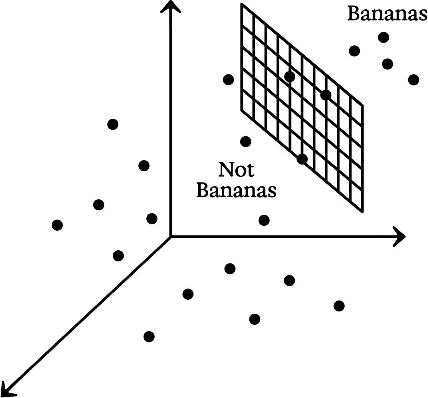
Conceptual sketch of a hyperplane separating points representing banana images from non-banana images
This “thresholding” transforms an embedding space that would otherwise be continuous into a categorical yes or no. A banana is either there or it isn’t. More precisely, if a banana is detected, that detection is invariant to whether the image’s banananess was just over the threshold or far over it. 3 Conversely, if the “no banana” neuron is activated, it doesn’t matter whether the banananess was just under the threshold, or far under it.
In summary, the transformation from the penultimate layer to the output layer consists of two steps. First, each output neuron is looking for a pattern in the previous layer (such as banananess), then the neuron applies a threshold to make that pattern detection more invariant. These are like the two kneading steps: rotating the ball of dough into a certain orientation, then pressing it down against a hard surface.
The same basic steps take place in every earlier layer of a deep neural net, too. All neurons calculate a weighted sum of activations in the previous layer. And although softmax is typically only used for the output layer, all neurons (artificial or otherwise) involve some form of thresholding or “nonlinearity.”
One of the most commonly used nonlinearities is ReLU, which stands for “Rectified Linear Unit”; such a neuron has zero response if the weighted sum of its inputs is less than zero, and otherwise has activation equal to that weighted sum. Like softmax (which, recall, approximates lateral inhibition in real neurons), ReLU is inspired by basic neuroscience. Real neurons either fire action potentials or don’t. Their firing rate is thus either zero or positive; a neuron can’t have a negative response. ReLU is pretty much the simplest nonlinear alteration one can make to the linear “identity function” f(x)=x to avoid negative output in an artificial neuron.
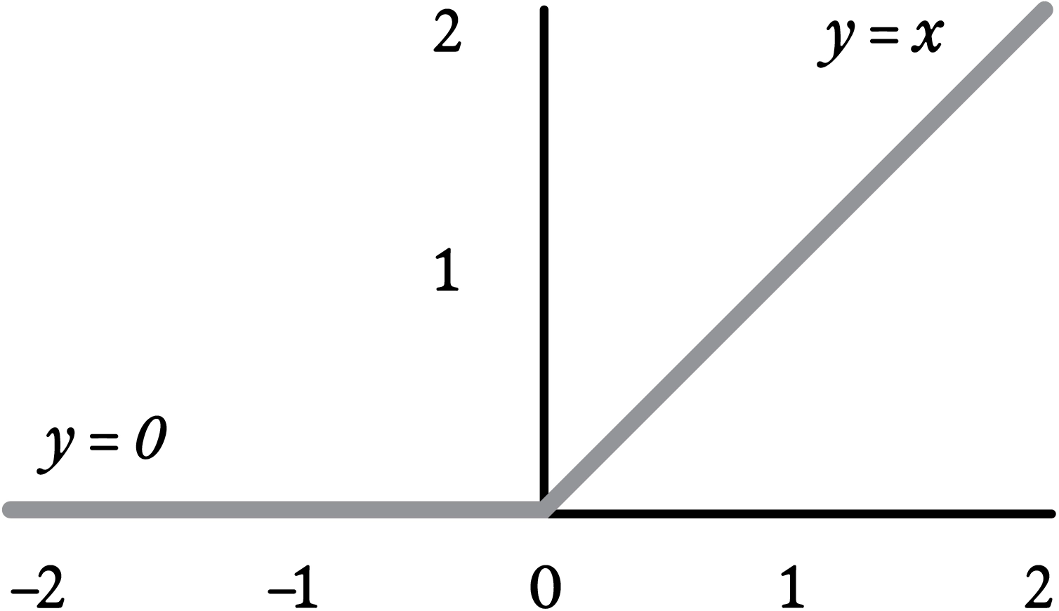
The ReLU (Rectified Linear Unit) nonlinearity
Nonlinearities like ReLU are essential to deep learning; without them, there would be little point in making a neural net more than one layer deep. A weighted sum of weighted sums is just another weighted sum. 4 However, with a nonlinearity, not only can successive layers no longer be replaced by an equivalent single layer, but, as mentioned in the previous chapter, virtually any function can be approximated, given enough neurons. 5
More intuitively, nonlinearities like ReLU implement a limited form of invariance. Every layer in a deep neural net is doing the same as the output layer: looking for a pattern in the previous layer and lighting up if it’s present. Single-neuron pattern detection is rudimentary, consisting as it does only of a weighted average—a form of recognition sometimes called “template matching.” Still, a neuron with a nonlinearity like ReLU turns the presence or absence of a pattern into an approximate “yes” or “no.” This allows the next layer to operate on higher-level, more abstract, and more invariant patterns.
To lean into the dough analogy a bit further, template matching, or taking a weighted average of the neural activations in a layer, is something like rotating the dough ball into a particular orientation. In fact, mathematically, it pretty much is a rotation—just imagine rotating the embedding space so that the hyperplane is horizontal, like a countertop. 6 Applying the nonlinearity then squishes the data down.
Without that squishing step, no useful work would get done by repeating the process—we would just be rotating the dough ball first this way, then that way, then the other way, which is equivalent to a single overall rotation. The squish between every rotation is what transforms the dough. There is no single rotation and squish that will produce the same result as a hundred consecutive rotations and squishes: the dough develops gluten, the network gets better at recognizing bananas.
Kneading dough … in reverse
The key difference is that when we knead dough, our rotations and squishes are random. We may have started with flour, water, and salt, but, by the end, these random operations have produced a uniform, glutinous output. Through the magic of machine learning, though, a trained neural network can do the opposite, starting with a “pixel dough” in which images of all kinds are swirled together, then progressively unswirling them until they’re cleanly separated by category. It’s as if, by orienting the dough just so before pressing it down each time, you could “unknead” it until you’re left with a big pile of flour, a little pile of salt, and a puddle of water.
Transfer
If we were to lop off the final softmax layer of our banana detector, its new output would be a 128-dimensional point in the embedding space of the previous layer. Given many varied input images, what kind of patterns would those points make?
It’s possible to visualize such patterns, although we must use mathematical tricks to reduce many dimensions down to something we can easily plot, in 3D or 2D. Many research papers have used such visualizations over the years, though the most striking one I’ve seen was made by a Turkish-American artist, Refik Anadol.
Refik Anadol’s Archive Dreaming AI data sculpture, February 2017
Already an established artist, Refik got his start in AI art with the Artists + Machine Intelligence (AMI) program my team and I founded in 2016, at the dawn of generative AI. He has since become famous. One of his first large-scale AI art commissions, Archive Dreaming, was a 2017 collaboration with SALT, an art and research institution based in Istanbul. SALT houses a major archive of photographs, architectural drawings, maps, posters, correspondence, and ephemera dating from the last century of the Ottoman Empire to the present, and they have been busily digitizing it. Refik used neural nets to generate embeddings for 1.7 million visual documents in the archive and created a room-size immersive visualization that allowed one to swoop through all of these documents, each rendered as a thumbnail hanging in the void. In that embedding space, visually similar objects cluster together, allowing one to get a sense of the archive as if it were a galaxy with 1.7 million stars, all arranged in space as if by a cosmic Dewey decimal system.
Suppose Refik had used the banana-recognition net to generate his embeddings, and the SALT archive had included a bunch of banana images. (For all I know, it might.) We know that a hyperplane would separate those banana images cleanly from the non-banana images; but what about other fruits, or other objects altogether? 7
Remember that the banana recognizer works by creating an increasingly invariant hierarchy of visual features; the banana/no-banana output neurons are just the visible tip of a submerged iceberg of features. Consider, for example, that unripe and overripe bananas look very different. Therefore different ensembles of features will likely have been combined to calculate one or more “banana of a certain ripeness” neurons in the embedding layer, but this ripeness information must be discarded to create the final ripeness-invariant banana neuron. The same will be true of bananas in different orientations, or under different lighting conditions.
These observations explain “transfer learning”: the ability to retrain a network to do a related task, using much less labeled data than would be required to train from scratch. 8 If we wanted our banana network to detect only ripe bananas, for instance, it would only take a bit of tweaking of those final 128 weights to exclude the unripe cases.
Caroline Dunn demonstrates the AIY Vision Kit, a Google product for experimenting with CNN-based on-device object recognition, in May 2018; note how, since pears are not part of the ImageNet dataset used to train this net, other visually related output neurons are activated.
More dramatically, the same trick will work nearly as well to turn the banana detector into an apple detector. Apples are also fruits, though red and round instead of yellow and long. The embedding layer will already contain neurons representing apple properties that are either like or unlike banana properties. Thus, apples could easily be detected simply by adding an apple neuron to the output layer alongside the banana neuron.
We could even learn the weights for that apple neuron from a lone exemplar, by setting them based on the activations of the embedding layer in response to a single apple image. 9 (An average based on a few apples would be better, but a single one will do.) The network will subsequently recognize “another of those.” 10 This is more or less what we do in adulthood when we learn about an unfamiliar object category from a single exposure. It’s called “one-shot learning,” and can be thought of as a special case of transfer learning.
The success of transfer and one-shot learning suggests that training a banana detector mostly involves getting it to learn how to see generically—that is, developing a general sense of perceptual invariance in the visual world. This involves learning the correlations between pixels in images, regardless of how those images are labeled.
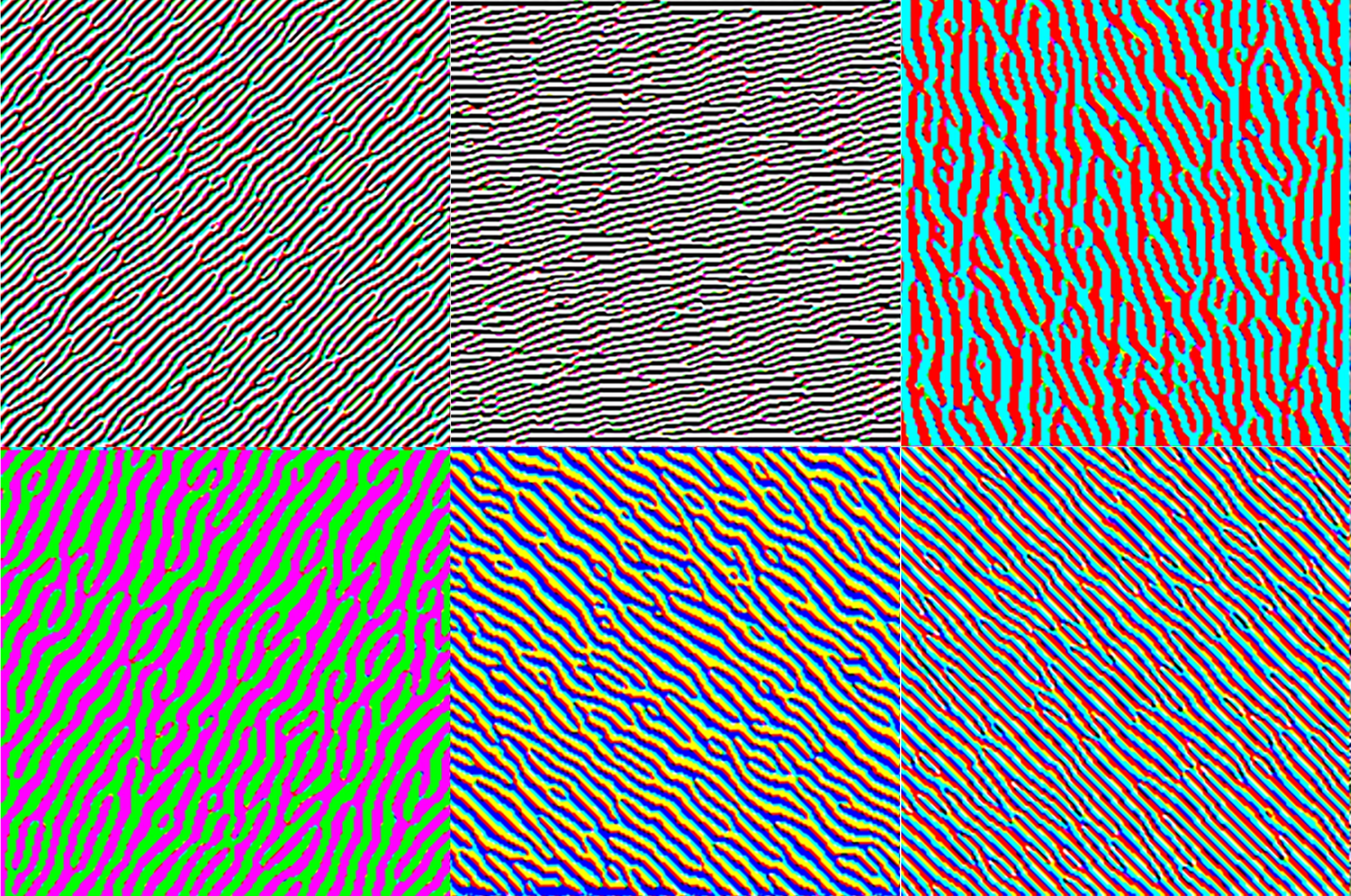
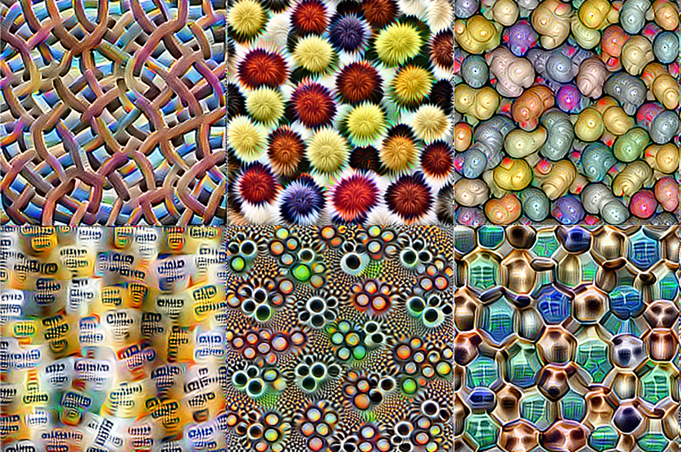
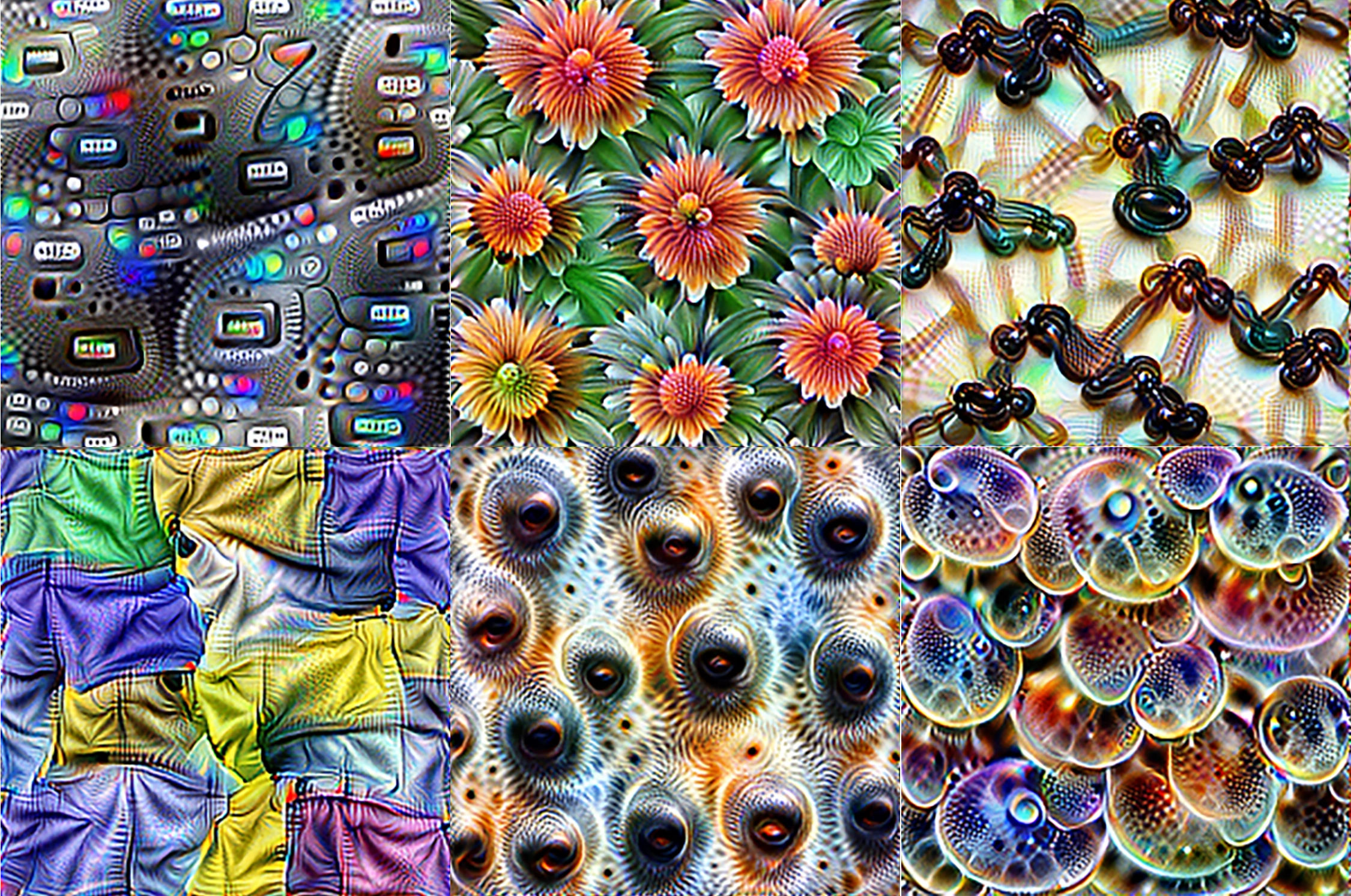
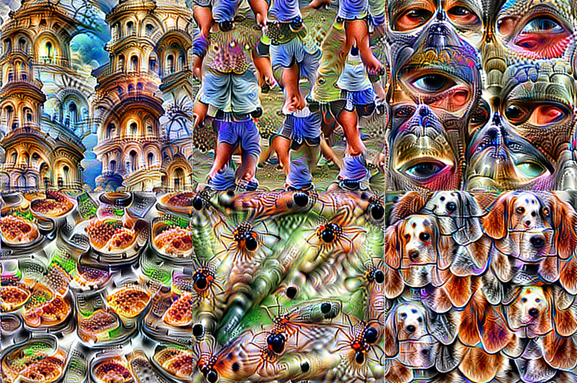
Images optimized to selectively activate specific neurons in different layers of a CNN. Neurons in early layers are sensitive to primitive features like edges, intermediate layers respond to textures and patterns, and later layers recognize semantically meaningful objects and object parts; from Olah, Mordvintsev, and Schubert 2017.
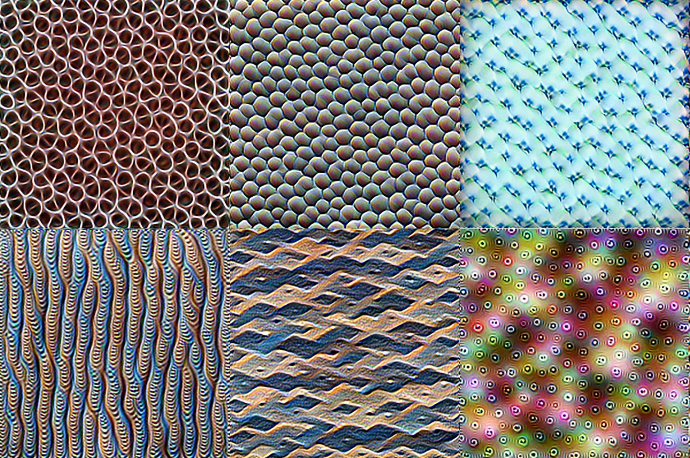
Images optimized to selectively activate specific neurons in different layers of a CNN. Neurons in early layers are sensitive to primitive features like edges, intermediate layers respond to textures and patterns, and later layers recognize semantically meaningful objects and object parts; from Olah, Mordvintsev, and Schubert 2017.
Images optimized to selectively activate specific neurons in different layers of a CNN. Neurons in early layers are sensitive to primitive features like edges, intermediate layers respond to textures and patterns, and later layers recognize semantically meaningful objects and object parts; from Olah, Mordvintsev, and Schubert 2017.
Images optimized to selectively activate specific neurons in different layers of a CNN. Neurons in early layers are sensitive to primitive features like edges, intermediate layers respond to textures and patterns, and later layers recognize semantically meaningful objects and object parts; from Olah, Mordvintsev, and Schubert 2017.
Images optimized to selectively activate specific neurons in different layers of a CNN. Neurons in early layers are sensitive to primitive features like edges, intermediate layers respond to textures and patterns, and later layers recognize semantically meaningful objects and object parts; from Olah, Mordvintsev, and Schubert 2017.
Is it necessary, then, to start with a banana detector at all? More to the point, do we really need to label a gajillion images with the banana/not banana bit to learn generic visual invariance?
We don’t. A neural network can learn how to see without any labeling. This simply means relying on unsupervised learning rather than supervised learning.
One popular unsupervised method, known as “masking,” involves blacking out random parts of the images and requiring the network to fill in, or “inpaint,” the blacked-out parts as accurately as possible. Any neural net that can do this well, for a large and varied set of images, will certainly have learned pixel correlations.
Notice that this is very much like predicting blacked-out words or passages in text—which is how large language models are trained! That’s why, in this book, I use the terms “prediction” and “modeling” almost interchangeably. To model data is to understand its structure, whether in space, in time, or both; hence, to be able to guess unseen parts of the data, whether those are masked or occluded in the present, or belong to the future (in which case the term “prediction” is most apt), or even took place, unobserved, in the past.
If a neural network has learned to successfully inpaint (or “predict”) missing pixels in a corpus of training images, that implies it has also learned how to recognize everything represented in those images—apples, fire hydrants, Siamese cats—not just bananas. It will know how to distinguish figure from ground, it will understand depth of field, it will recognize colors, and it will be able to distinguish ripe from unripe fruit. The evidence: if the network was trained on banana images, and you test it by blacking out half of a previously unseen banana image, it should convincingly fill in the other half. Moreover, the ripeness of the filled-in half should match the ripeness of the visible half.
This raises some interesting questions, both practical and scientific. On the practical side, all sorts of knowledge may be latent in a neural net trained with unsupervised machine learning, but how would we read it out? That is, how could one turn this pixel inpainting model into an actual Siamese cat detector, banana detector, or fruit-ripeness detector?
We might also wonder about the relationship between unsupervised learning and neuroscience. It’s nice to get rid of all that banana/not banana labeling, but blacking out random regions of a sheaf of arbitrary images and training the model to fill them in still seems like a highly artificial task. What does this have to do with how learning works in brains?
Green Screen
The limitations of transfer learning, and the parallel limitations of our own brains, are revealing. If the banana network had been trained entirely on photos taken in supermarkets and we then tried to use it to recognize individual faces, it would do a poor job, because the transformations leading to the embedding layer would not include learned representations of the needed features. Even if supermarket shoppers had been visible among the “not banana” images, the relevant details of their faces might get discarded early in the network, because those details are irrelevant to banana detection—if it’s any kind of face, it’s not a banana, end of story.
A similar effect explains why people who grew up in a racially homogenous environment tend to be so poor at distinguishing individuals of other races. We learn our face embeddings young, and they are exquisitely sensitive—but only within the statistical distribution we have learned from. Hence the all-too-common sayings, usually considered racist, that all people of a “foreign” race “look alike.” 11 Yet in a very literal sense, if our brains weren’t exposed to “foreign” faces as children, then, for us, it’s true. As adults, the best we can do is to understand the limitation and work on it (ongoing improvement is possible 12 ). Less excusably, the same problem is evident in convolutional nets trained to recognize faces based on inadequately diverse datasets. 13
The same phenomenon holds for recognizing phonemes. In Japanese, for example, there are no separate “r” and “l” phonemes, making it hard for adult native speakers to distinguish between the English words “rock” and “lock.” Studies dating back to the 1980s and ’90s show that, from the moment an infant’s brain is exposed to language—and long before learning to speak—the brain’s neural networks begin to learn meaningful invariant representations of speech sounds. 14
While these invariant representations constrain what the baby can hear (and later, say), they are essential “scaffolding” for learning higher-order concepts. In particular, babies can learn new words efficiently only once they have developed a rich lower-level representation of the necessary speech sounds. Japanese adults learning English can, over time, improve their ability to discriminate “r” from “l,” but it’s much more of a slog than learning a new word in Japanese, since learning a new low-level representation doesn’t benefit from any of that developmental scaffolding.
Learning, then—whether supervised or not—is mostly a matter of “representation learning”—that is, learning how to embed. Using a combination of theory and machine learning experiments, physicist and AI researcher Brice Ménard and colleagues have demonstrated that representation learning in multilayer perceptrons is universal, regardless of how they’re trained. 15
One could even say that learning is also learning to learn. That is, once a suitable generic embedding or representation has been learned, associating a label with a specific point or region in the embedding space becomes trivial.
So, although our brains take a long while to learn how to see the world and how to hear language, once we have these representations down, we become adept one-shot learners. If you are shown a kiwi for the first time, you’ll henceforth immediately be able to recognize that furry little fruit. A perceptron trained on general vision tasks can do the same, with the addition of a kiwi neuron to the output layer trained in one shot. That’s so much easier than labeling lots of kiwi (and not-kiwi) images and training on them from scratch.
If a perceptron is trained to inpaint pixels rather than detect bananas, its high-level layers will be general embeddings, equally good at representing bananas, faces, cats, kiwis, and anything else in the (unlabeled) training data. Moreover, there will be neurons specifying the ripeness of fruits, the features of faces, and the breeds of cats. When the image is of a cat, its eye color will be guessed if need be, for instance if we’ve blacked it out—otherwise, those pixels could not be filled in. It follows that latent eye-color knowledge is also present if the cat happens to be facing away from the camera.
You can see how powerful unsupervised learning is. That’s why, in recent years, researchers have been shifting away from the old supervised approach. Not only are the large numbers of labels we used to rely on unnecessary; they may actually impede learning, since training a model only on a particular classification task can allow the learned representations to get away with being less robust. Moreover, the very fact of labeling is bound to introduce additional errors and biases, and is also labor intensive—at best, boring, and at worst, exploitative. 16
The hourglass-shaped “masked autoencoder” is now a common way to construct an unsupervised perceptron-style model. 17 Starting from a “retinal” input layer of, for example, 512×512 color pixels, a sequence of progressively narrower layers culminates in a bottleneck—say, 128 values—which then expands back into an output layer of the same shape as the input. The input omits masked pixels, which may amount to seventy-five percent of the total, while the output reconstructs (or “hallucinates”) the whole image.
Masked autoencoder demo; He et al. 2021.
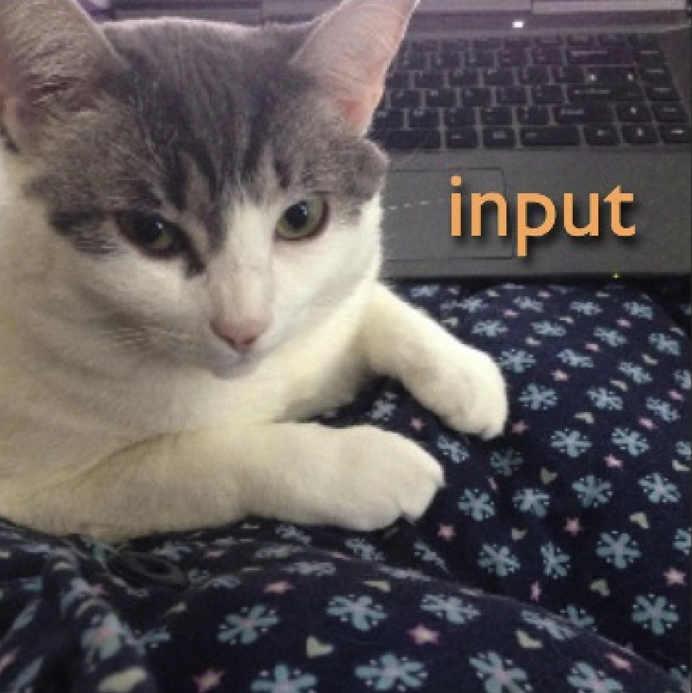
A masked autoencoder might appear unimpressive. If you picture it as a machine with a digital camera connected to the input layer and a display connected to the output layer, it seems to behave like an ordinary viewfinder. You feed in a 512×512-pixel image of a Siamese cat, and out comes … a 512×512-pixel image of the same cat, indistinguishable at a glance from the input.
The masking capability adds magic, though. In addition to the three color channels (red, green, and blue), masked autoencoders use a binary masking channel to tell the network which pixels to use as input, and which to inpaint. Suppose you dipped your hand in a special color of green paint that will be interpreted as that mask—as in the “green screening” technique in Hollywood, where live actors are recorded against a solid-green background in the studio, then the footage is composited into a computer-generated environment. Here, you’d wave your green-painted hand in front of the camera, and the autoencoder would do its best to inpaint those pixels. On the viewfinder, anything that shade of green would be invisible, as if the autoencoder had perfect x-ray vision and could see right through your hand—even if you were to cover a large portion of the visual field.
Of course, that inpainted content is a hallucination. If the area you cover up is small, or is entirely predictable from the surrounding context, the reconstruction will seem flawless. But in general, it won’t be. If your hand is partly occluding the cat’s body, there’s no way for the model to know the arrangement of every hidden strand of fur, so those details will be made up. And if you cover everything except a corner of blue sky, the reconstructed scene might have little in common with what’s actually there.
The first half of the neural network begins with an input image and, layer by layer, narrows to 128 values at the bottleneck. It looks just like a supervised classifier stripped of its output layer, which suggests that the bottleneck acts like an embedding—and indeed it does.
We can also interpret the bottleneck layer as a form of image compression (as described in chapters 1 and 2). Compression is, in a deep sense, closely related to language. It extracts the meaning from a signal, its semantic essence, from which the original can be reconstructed, at least statistically. If you can see just enough of the cat’s body to know it’s a Siamese, then this knowledge suffices to imagine what its head will look like, where its eyes will be, and that those eyes will be blue. The strands of fur might all lie in different places in the reconstruction, but if it’s done convincingly, a judge confronted with the original and the reconstruction wouldn’t be able to guess which is which. The details would vary, but the semantic content would be the same.
Grandmother Cell
Our visual cortex is not so unlike a perceptron, but it doesn’t get trained by reconstructing arbitrary collections of partially masked static images. Instead, our brain is exposed to a continual stream of “video” from our eyes, broken up by eye movements, called saccades, that we make approximately five times a second. The brain also controls those saccades, along with the orientation of our heads and the position of our bodies, so the stream isn’t passive, but actively generated.
Still, masked-autoencoder training isn’t as far from our experience as it may seem. The retinal fovea, where we can resolve enough detail to read, is barely big enough to make out a handful of printed words. Even that region is noisy and jittery. The wider visual field is much lower in resolution and crisscrossed with blood vessels. 18 This certainly differs from our impression of what we see.

Under controlled experimental conditions—viewed at the appropriate distance through a single eye fixated on the dot in each—these synthetic images are visual “metamers,” meaning they are indistinguishable from an undistorted version of this page of text from Moby-Dick. This illustrates the relatively small area around the fovea where we can clearly resolve detail; from J. Freeman and Simoncelli 2011.
A dramatic series of experiments using eye tracking done in several labs between the 1970s and the ’90s illustrates this. 19 A subject sits in front of a display showing a grid of letters. Wherever the viewer’s eyes are looking, the display shows stable underlying text, but everywhere else, the letters are randomized. To an onlooker, the entire screen looks like an illegible jumble. But, if the window of clear text is a mere eighteen characters wide—about three characters to the left of the fixation point and fifteen to the right, in a language like English that is read from left to right—then to the subject, the whole page of text looks clear and steady. This is what neuroscientists mean when they say we “hallucinate” the world into existence based on the sketchiest of signals.
From the moment we open our eyes, soon after birth, and begin swiveling them around using our “exterior ocular muscles,” we’re putting our visual systems through an unsupervised training regimen much like that of a masked autoencoder. With every saccade, we have the opportunity to test whether or not a previously unresolved part of the environment looks as we had predicted or “inpainted” it in our heads, and to improve our model accordingly.
Eye-tracking study of a young child reading; at this age, the eyes dwell on each word, while more advanced readers saccade rapidly over whole phrases and sentences, taking advantage of their more developed predictive models of text
After a while, we learn to saccade to the spots that matter the most, and where our uncertainty is highest—was that a tiger nosing through the underbrush?—thereby constantly pinning our reconstruction to reality. Of course, the moment we saccade away, uncertainty in that spot begins to grow again, reminiscent of the way an unobserved particle begins to blur in quantum mechanics.
Vision is not the raw stream of sensory input from our eyes. Rather, that input stream acts like an error-correction signal. Vision—what we actually see—is a reconstruction of the world around us, an actively maintained and constrained hallucination.
Using nothing but prediction, then, we will rapidly learn a powerful unsupervised model of our visual environment. It will include sparse neural representations that have just the kinds of high-level semantic meanings that masked autoencoders learn, that Hubel and Wiesel recorded in the cat visual cortex, and that have even been recorded from the brains of awake humans. 20
A “grocery trip” generated by processing video using Alex Mordvintsev’s Deep Dream algorithm, which alters image pixels by partially “hallucinating” their values through the enhancement of activity in the semantic layers of a CNN; Mordvintsev, Olah, and Tyka 2015. Suzuki et al. 2017 hypothesize that hallucinogenic experiences are similarly a result of heightened top-down prediction at the expense of bottom-up error correction.
I introduced the concept of sparsity in chapter 3 to describe connectivity in neural networks, both artificial and biological. In a sparse network, neurons are only connected to a small subset of the other neurons in the net; unless the network as a whole is very small, this constraint is essential for efficient learning—and, in a real brain, it is physically impossible for every pair of neurons to be connected. The whole field of deep learning can be understood as an exploration of sparse neural architectures, starting with the separation of neurons into multiple distinct layers.
The idea of sparsity can extend from connectivity to activity. 21 In a neural network with sparse activity, only a small subset of neurons will be active (that is, have nonzero activation) at any given time. This, too, is a physical requirement for biological brains, because a neuron burns serious energy when it fires. (That’s why epileptic episodes, in which overexcited populations of neurons start to fire continuously, can’t go on for too long, and can lead to brain damage as energy reserves deplete and toxic byproducts build up.)
Even without such physical constraints, sparse activity appears to arise naturally in trained neural networks. 22 In the final layer of a classification network, the reason is clear: softmax forces the output layer’s total activity to sum to one, while supervised classification encourages a one-hot distribution, with the activity dominated by a single neuron—an extreme form of sparsity.
Less obviously, activation sparsity emerges in earlier layers too. Nonlinearities like the ReLU function naturally lead to sparsity, since they replace what would otherwise be negative activity with zero activity, and the resulting “quietness” in one layer spreads through subsequent layers. But in a more profound sense, sparse activity comes with the increasing specificity of every neuron’s response as the network learns. 23
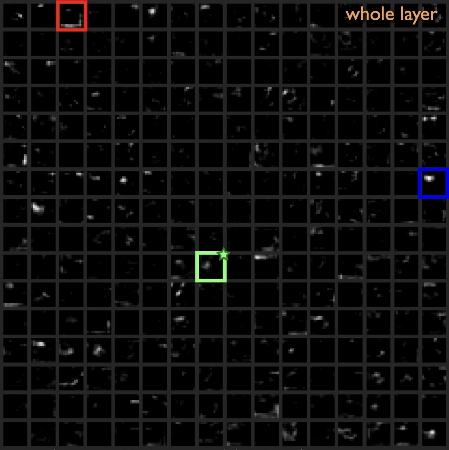
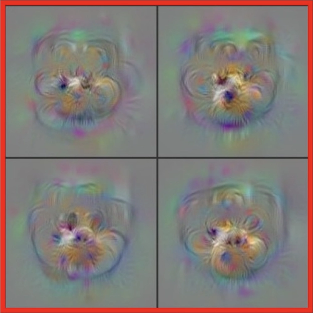
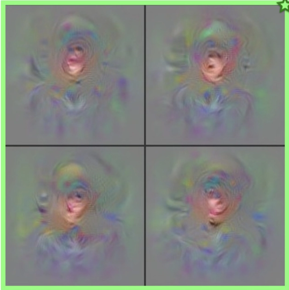
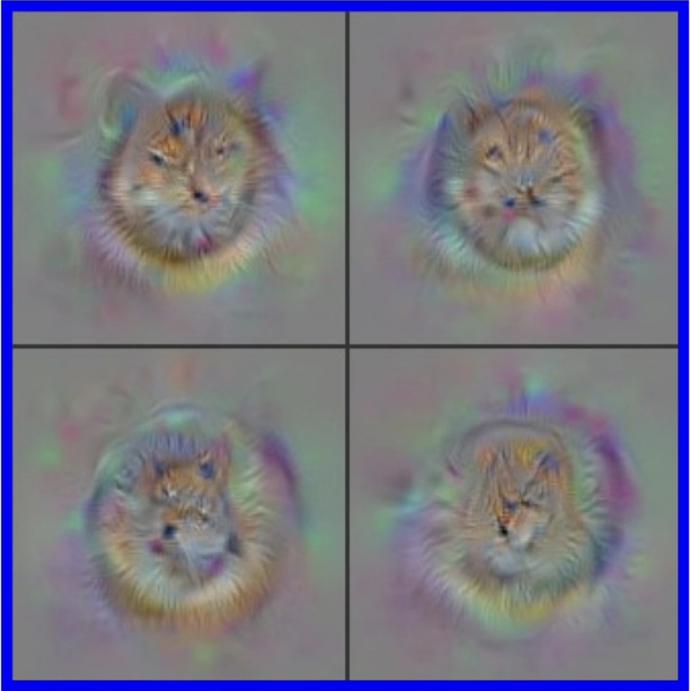
Sparsity of the activations of units in a CNN in response to a natural image. Visualizing the features producing these sparse activations reveals that they are often mixed or complex: the neuron in the red box responds to dog faces and flowers; the neuron in the green box responds to human and cat faces; and the neuron in the blue box responds mainly to cat faces, implying sparse but not one-hot coding in these intermediate layers; Yosinski et al. 2015.
Sparsity of the activations of units in a CNN in response to a natural image. Visualizing the features producing these sparse activations reveals that they are often mixed or complex: the neuron in the red box responds to dog faces and flowers; the neuron in the green box responds to human and cat faces; and the neuron in the blue box responds mainly to cat faces, implying sparse but not one-hot coding in these intermediate layers; Yosinski et al. 2015.
Sparsity of the activations of units in a CNN in response to a natural image. Visualizing the features producing these sparse activations reveals that they are often mixed or complex: the neuron in the red box responds to dog faces and flowers; the neuron in the green box responds to human and cat faces; and the neuron in the blue box responds mainly to cat faces, implying sparse but not one-hot coding in these intermediate layers; Yosinski et al. 2015.
Sparsity of the activations of units in a CNN in response to a natural image. Visualizing the features producing these sparse activations reveals that they are often mixed or complex: the neuron in the red box responds to dog faces and flowers; the neuron in the green box responds to human and cat faces; and the neuron in the blue box responds mainly to cat faces, implying sparse but not one-hot coding in these intermediate layers; Yosinski et al. 2015.
Sparsity of the activations of units in a CNN in response to a natural image. Visualizing the features producing these sparse activations reveals that they are often mixed or complex: the neuron in the red box responds to dog faces and flowers; the neuron in the green box responds to human and cat faces; and the neuron in the blue box responds mainly to cat faces, implying sparse but not one-hot coding in these intermediate layers; Yosinski et al. 2015.
Your cortex doesn’t have any single “banana” neuron. However, the idea that we might have unique neurons in our brains corresponding to highly specific percepts or memories has a long history. The term “grandmother cell” was coined in 1967, somewhat cheekily, to refer to a hypothetical neuron that activates only in response to one’s grandmother. 24 Margaret Livingstone’s recollection of a cat visual neuron that, after an extensive search, was found to respond only to a yellow Kodak film box can be interpreted as evidence of something resembling a grandmother cell. A famous 2005 Nature paper, “Invariant Visual Representation by Single Neurons in the Human Brain,” 25 documented a neuron in a human subject that seemed to respond only to Jennifer Aniston … and another neuron that responded only to Jennifer Aniston and Brad Pitt together! 26 The researchers also found a Pamela Anderson neuron, which responded specifically not only to pictures of Anderson (including a caricature of her), but also to her name written out—and not to any other name or string of letters they could find.
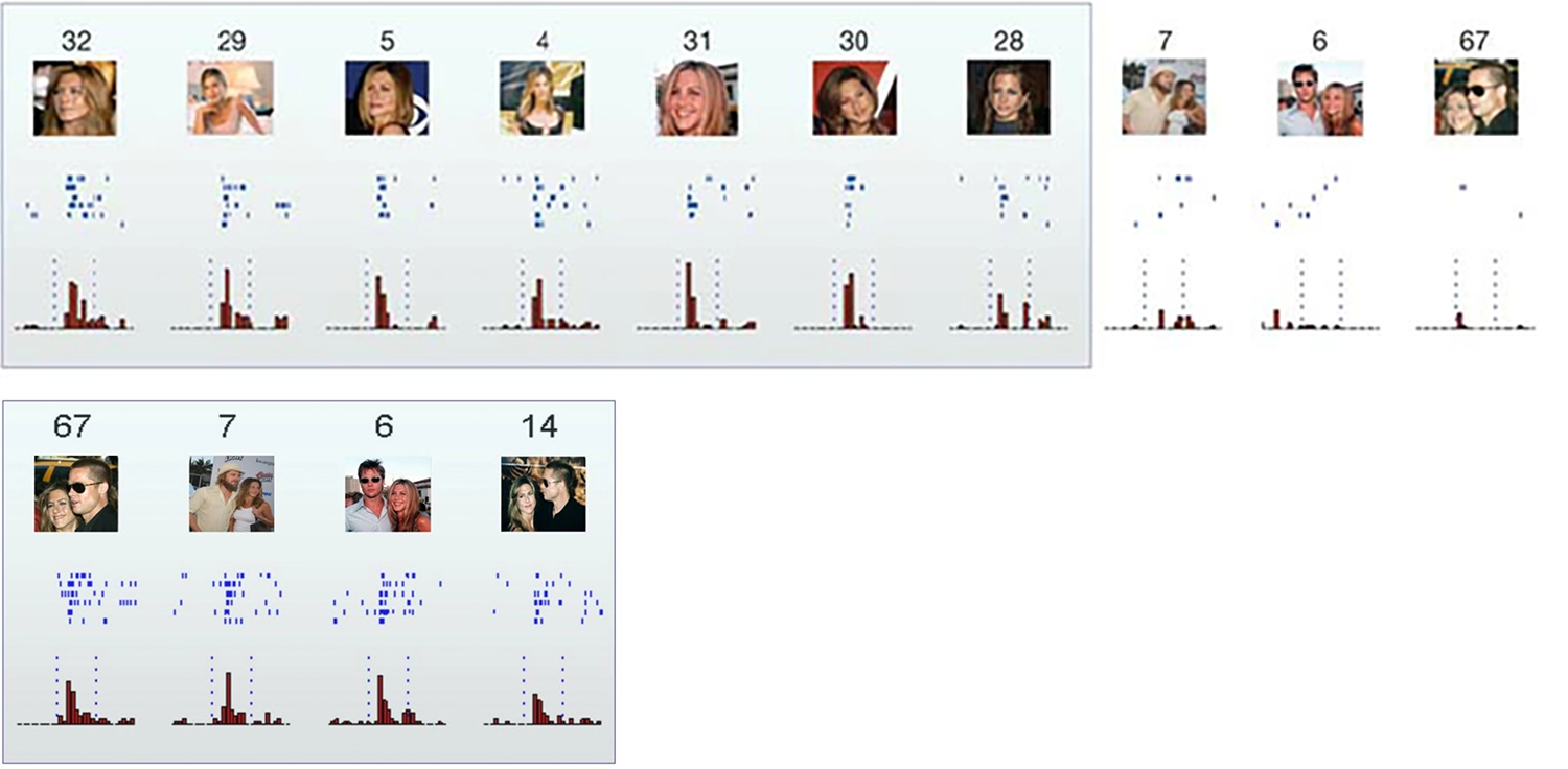
Responses of single neurons in the hippocampus to a selection of the eighty-seven pictures presented to a human patient. The first neuron fired to all pictures of Jennifer Aniston alone, but not (or only very weakly) to other famous and non-famous faces, landmarks, animals, or objects. Neither did the neuron respond to pictures of Jennifer Aniston together with Brad Pitt—though another neuron (bottom row) fired only in response to the pair; Quiroga et al. 2005.
As suggestive as these findings are, remember that no supervised-learning process was forcing a (hypothetical) one-hot layer somewhere in your brain to activate a single “banana” or “grandmother” or “Pamela Anderson” neuron, to the exclusion of all else. Such single points of failure would make your brain far too fragile. Would you suddenly be unable to recognize your grandmother if “her” neuron died one day, or just failed to fire? And if you’re using up neurons on such granular concepts as Jennifer and Brad together, do you risk running out?
No: in a sparse distributed code, which is learned by a set of high-level neurons (analogous to the embedding layer) with neither supervision nor centralization, a whole set of neurons in your brain lights up in response to your grandmother, or a banana, or a specific movie-star couple. Even if only one in ten thousand light up, that’s still nearly ten million neurons. So if a few of those remain silent, it probably won’t matter. (And, while the code is sparse, it’s not too sparse, or a neuroscientist poking around in someone’s brain while showing them pictures would never get lucky enough to find a Pamela neuron, let alone also a Jen neuron, and even a Jen and Brad neuron.)
An artificial neural network decoding neural activity from a mouse’s visual cortex is able to estimate which frame of a video the mouse is looking at; Schneider, Lee, and Mathis 2022.
As a bonus, sparse distributed representations are vastly more efficient than a one-hot code. With 128 neurons, a one-hot code can only represent 128 things. In a sparse code that involves, say, sixteen of them lighting up at a time, there are about ninety-three quintillion possibilities. 27 With larger numbers of neurons, the available combinations are virtually limitless, even accounting for plenty of redundancy.
Final Causes
Let’s now switch from a perception-centric to a motor-centric perspective. In doing so, we will be moving farther away from perceptrons and closer to real critters.
Suppose a neuroscientist records from neurons somewhere along the complex pathway from an animal’s visual cortex to its exterior ocular muscles, postulating, quite reasonably, that these spike trains (that is, sequences of action potentials) issue motor commands for eye movement. How could the neuroscientist “decode” this command stream? The answer, of course, is to simultaneously measure eye movement and build a model (these days, probably using an artificial neural net) that, given the spike trains, can predict eye movement. If it works reasonably well, voilà—an eye-movement command-stream decoder, and thereby proof that what is being recorded is a command stream!
However, what the neuroscientist has actually created could equally be interpreted as an artificial brain region that—if the predictive-brain hypothesis is right—performs exactly the same kind of prediction task that every other brain region performs! The “decoding” will “work” reasonably well, to the extent that
- most of the information used by downstream neurons to carry out their prediction is captured by the recording,
- the timescale is fast enough to allow feedback loops to be ignored,
- the neuroscientist’s model is sufficiently powerful to proxy the downstream brain region, and
- the downstream region isn’t actively trying to evade prediction via dynamical instability and randomness (per chapter 3).
In short, given the feedback loops present everywhere in the brain, the “command stream” interpretation is arbitrary. If various brain regions are trying to predict each other, no inherent hierarchy determines which one is giving orders.
Placing a fruit fly in a virtual reality environment while recording from its brain allows experimenters to build artificial neural networks to decode aspects of the animal’s motor activity and world model; Seelig and Jayaraman 2015.
Neuroscientists and AI researchers may find this counterintuitive; we need a bit of neuroanatomy to understand why. Neurons have a cell body located near the “dendrites” that receives inputs, and a long process, the “axon”—I’ve previously called these connections “wiring”—sending neural spike trains to other neurons (or muscles) elsewhere in the brain or body. Those wires can be really long. For instance, the axon of a motor neuron with a cell body in the lumbar region of your spinal cord can extend all the way to the tip of your big toe, a distance in excess of three feet. (In blue whales, axons can be thirty feet long!)
It’s tempting to imagine neurons as little people, doing their “thinking” near the body or “head” and deciding what signal to send out along their axonal “tail” to a downstream target. Using philosophical language, one could say that we think of the head as the “agent” and the tail as the “patient,” meaning the passive recipient of the agent’s actions. 28
The idea that the target could be in charge seems odd, given where the decision about when to spike appears to be made and the direction in which that spiking signal appears to travel. But, in a sense, the tail wags the dog.
An example will help illustrate why. Imagine a theater has fifty free seats that become available five minutes before a show starts, at eight o’clock sharp. The usher is given a counter. At 7:55, she starts pressing its button every time someone walks in so that she can close the doors when the counter reaches fifty, or at eight o’clock, whichever comes first. It’s a popular show, so at 7:57 the doors close.
Why did the doors close? One answer, corresponding to what Aristotle called the “efficient cause,” is that the fiftieth person walked through the door. Another, deeper answer, corresponding to what Aristotle called the “final cause,” is that the theater had reached capacity. These “whys” differ in where they locate agency.
If we were alien researchers studying the theater, we would notice that a particular person walked through, triggering a click, causing the usher to close the doors, and could easily mistake that fiftieth theatergoer for the agent that made the doors close. The aliens would, in other words, observe a “command stream,” with the commands issuing from the theatergoer to the usher.
But, of course, none of the theatergoers exhibited agency here. The fiftieth theatergoer might not even have noticed that he was the last one to make it in, and certainly would not think of himself as having closed the door. To understand where the agency really lies, we need to zoom out and look at the whole system from a functional or purposive point of view, and this requires understanding events farther back in time—the causes of the causes—as well as more abstract concepts like theater capacity and the usher’s job description.
As every kid knows who has asked an increasingly annoyed adult “why” after every attempt at an explanation, there really is no such thing as a final final cause. It is meaningful, though, to distinguish between a mechanistic or “how-like” why and a purposive, agential, “final cause” why.
Here’s one way to tell the difference: when an event has a final cause, disrupting the causal chain leading up to it will (when possible, and within limits) not permanently disrupt the event, but merely force it to be achieved by other means—which implies an intelligent agent at work, doing that “causal rerouting.” For instance, if the theater-observing alien is meddlesome and takes away the clicker, the usher will shrug and use some other method to count people as they come in, perhaps with marks on paper or a mental tally.
Similarly, if one of your muscle cells is working hard and there isn’t enough oxygen available to meet the energetic demand with aerobic respiration, it will switch to anaerobic metabolism, a different set of chemical pathways that can liberate free energy without oxygen. Agents are adaptive and resourceful, even when they are individual muscle cells!
Hence it’s meaningful to answer the question “why do our cells need oxygen?” with the final cause answer, “because it’s used to obtain free energy.” 29 Oxygen is needed for the aerobic means to that end, and obtaining free energy is a critical cellular function that must be achieved one way or another. (Unfortunately, in our cells, an oxygen debt is incurred via the anaerobic route, so you can’t remain anaerobic for long, and you’ll pant for a while after the vigorous exercise stops.)
Now let’s return to the nervous system. Neural circuits are functional too, and, in complex nervous systems, their functions are learned. Learning requires signals relating activity to its downstream effects to flow backward, from target to source; hence the “backpropagation” algorithm for training artificial neural nets. As will be discussed in chapter 7, real brains are unlikely to implement the backpropagation algorithm, but whatever algorithm they use must involve information about “downstream” effects somehow making its way back “upstream” to the neural machinery that caused those effects, so that the machinery can be modified accordingly. In this sense, learning is the very essence of backward causality.
Neuroscientists often don’t directly observe learning taking place in electrophysiological experiments, because it’s slower than real-time electrical activity. It’s also not nearly as well-understood. We figured out how neurons spike in the 1950s, but are still arguing about how they modify their inputs and parameters to learn when to spike. Hence, our understanding of the slower aspects of nervous systems exhibiting backward causality lags far behind our understanding of the mechanisms underlying their rapid, forward causality.
More abstractly, we tend to notice only efficient causes, and not the final causes, just as an alien watching the theater fill up would have missed the earlier interaction when the theater manager gave the usher a clicker and directions about when to close the doors.
Sometimes final causes get ignored for another, related reason: they smell of teleology. Indeed, the whole idea of a final cause only makes sense in the context of purposive behavior. But as we’ve seen, biological (and more broadly “entensional”) systems are characterized by purposes. We can only understand them functionally, which means embracing Aristotle’s final causes.
Meathead
This brings up an unsettling question: to what degree is the brain really “in charge” of the rest of the body?
Since learning determines what each neuron does—which signals it responds to and which it ignores—a neural cell body with a long axon projecting to a different brain region doesn’t only live to serve the region near the cell body. It’s also an outpost, a listening station, whose learned function involves serving the community of neurons at the far end of the axon.
This is most obvious for the neurons in our sensory periphery, which we can think of as being in contact with our environment. Pressure and temperature sensors in our skin relay their signals to “somatosensory” cortex; light-sensitive cells in our retinas send information to the visual cortex; and vibration-sensitive hair cells in our inner ears send information to the auditory cortex. 30 These cells are clearly information-gathering outposts.
You probably wouldn’t say that a sensor on your fingertip is the “boss” sending commands to drive your behavior, but, rather, that it’s one of many inputs informing your behavior. Under certain circumstances, though—such as touching a hot stove—it would be hard to argue that these sensory neurons aren’t bossing you. Your interests as an organism are best served by the fastest possible reaction time, pushing initiation of this action as close to the source of the signal as possible. So your brain doesn’t decide, but is merely informed about what you did after the fact.
Retraction reflex of a snail’s tentacles
What about the muscular end of things? This is where the usual “brain in charge” picture seems least in question. The idea of our brain being in charge of our muscles seems obvious, while the idea of our muscles being in charge of our brain sounds, on the face of it, absurd. As everybody knows, brains are smart and muscles are dumb; otherwise, “meathead” might be a synonym for “genius.”
Indeed, on their own, muscles are seemingly passive. That’s why, if you get a nasty knock on the head, you will fall down. While you’re unconscious, your muscles will go limp and do nothing. Your body will be like a marionette with its strings cut.
Or will it? Despite its intuitive appeal, this view may be too one-sided. Consider your heart, gut, and blood vessels—they’re muscles too. Luckily, they don’t stop contracting when you’re unconscious or asleep. The heart can continue to beat rhythmically for quite a while, even when disconnected from the brain.
A human heart, kept alive for a transplant procedure, continues to beat on its own
Indeed, the earliest motile life forms, dating back at least to the Ediacaran (635–538.8 million years ago, just prior to the Cambrian), didn’t have centralized nervous systems at all, but they certainly had muscular coordination. Muscles are useful even for the simplest “sessile” animals—those anchored to rocks on the seafloor—as they allow rhythmic pumping movements to filter seawater over or through their bodies to sieve out nutrients. Jellyfish perform such rhythmic pumping while free-floating, enabling them to swim.
Coordinated oscillation can occur at larger scales and among more complex organisms, too. Giant swarms of certain firefly species, for example, can glow in near-unison, creating an otherworldly Christmas light spectacle. 31 Both the synchrony of a firefly swarm and the speed with which they can get into sync depend on the ability of the fireflies to see each other. They’re able to coordinate quickly—and stay coordinated—because they can see not only their immediate neighbors, but also the glow of more distant fireflies, halfway across a clearing. 32
Whether the oscillators are individual muscle cells or whole fireflies, coordination requires a flow of information, but it need not involve any centralized control. We can think of what the individual units are doing as a minimal kind of local prediction, or pattern completion. Each unit aligns the frequency and phase (i.e., timing) of its oscillation with that of its neighbors. At the most basic level, coordinated movement is what makes many entities into one.
The freshwater polyp Hydra
“Phase synchronization” is the way the heart works too. Peristalsis—the coordinated toothpaste tube–squeezing maneuver that moves food along the gut—similarly relies on a traveling wave of contraction. Decentralized coordination among muscle cells in organs like the heart and gut, and in animals like jellyfish and Hydra, is partially achieved via “gap junctions”: channels that couple two neighboring cells, causing electrical activity in one to propagate directly into the other. However, fast and efficient synchronization of muscular contraction requires longer-range connectivity. The decentralized nerve nets of jellyfish and Hydra provide such long-distance connectivity, just as the visual systems of fireflies allow them to coordinate across that forest clearing.
In fact, some of the earliest neural nets appear not to be made of distinct neurons at all. The “subepithelial nerve net” of the comb jelly, an ancient branch of animal life dating back to the Ediacaran, consists of a fused or “syncytial” network of nerve fibers, effectively serving as an undirected, organism-wide highway for long-distance information transmission. 33 Perhaps these earliest neural nets are best thought of as providing extended internal sensory systems for muscle cells, allowing them to contract in synchrony with faraway neighbors. 34
The common northern comb jelly, Bolinopsis infundibulum
How and why, then, did organisms with diffuse neural nets evolve centralized brains? A likely answer: sensing the external environment is helpful for muscle cells too.
Food, of course, is an all-important environmental signal. And pretty much everything that is alive pulls away from noxious stimuli, just as our hands do from a hot stove—in general, using a fast, local feedback circuit. Chemical receptors—implementing chemosensing, or what we call “taste”—are in turn the oldest and most ubiquitous environmental sensors, capable of detecting both yum and yuck. Recall that even bacteria have such sensors, since in a watery medium and at the smallest scales, floating molecules are the environment.
Now, consider the saliency of such receptors for an animal that can both propel itself forward and turn via rhythmic muscular contraction—something worm-like, for instance. While a coral polyp lives anchored to one spot and must make the best of whatever washes over it, a crawling worm continually makes decisions that will determine its future environment, hence its survival prospects. In this respect, it resembles a swimming bacterium.
Sea squirts (Ascidiacea) possess a central nervous system during their free-swimming larval stage, but reabsorb most of it when they attach to a substrate and transform into their sessile adult form: there is no point in having a brain for an animal that is no longer motile.
Unlike a bacterium, though, a worm is long and bilaterally symmetric, or “bilaterian,” rather than tiny and cylindrically symmetric. As a result, it can steer left or right, not just run or tumble—an innovation critical to life on land. As philosopher and naturalist Peter Godfrey-Smith has pointed out, “In the sea, animals have various body plans. On land, all animals are bilaterian. There are no terrestrial jellyfish.” 35
Receptors at the front end of a bilaterian are especially important, because they’re the first to detect an encounter with anything tasty or aversive. That is, unlike a coral, a bilaterian moves through the world in a particular direction, so it has a leading end. And unlike the point-like bacterium, space and time are meaningfully correlated; one could say the front end of a worm lives in its future, while its rear end lives in its past. Muscles throughout the body will need to know about the future, and the ones on the right and the left will want to behave differently in order to turn away from noxious things and toward food.
Acoel worm of the family Dakuidae
Thus, a symbiotic partnership emerged between muscle cells and their non-motile, spatially extended cousins, nerve cells. The usual way of thinking about this partnership holds that the neurons took control of the muscle cells, but I’ve argued that it may be equally valid to think of early neurons as information conduits, or even as sensory outposts, to serve muscle cells. Initially, neurons allowed improved long-range coordination across the body. But by wiring up preferentially to the leading end of the animal, muscles could also respond to any important changes in chemical concentrations up there.
Among bilaterians, those responses needed to be differentiated from the start, not only by stimulus type, but also by stimulus and muscle location. A “yum” to the right, or a “yuck” to the left, should cause the muscles on the right side, but not the left, to contract. It’s not so easy for a diffuse neural net to convey such spatially differentiated signals.
So, as muscles all over the body began to wire up selectively to the front end of the animal, the resulting knot of spatially organized neurons resulted in “cephalization”: the first glimmers of a brain in the head.
Neuromodulators
In addition to growing simple brains to support immediate perceptual input, bilaterians immediately faced a need to modulate their behaviors on timescales longer than the activations of individual neurons or muscles. Even chemotactic bacteria need to compute a “batting average,” adding up, or integrating, what they sense over a long period to decide whether the food level in the environment is going up (in which case they should keep swimming), or down (in which case they should tumble and change direction). Bilaterians needed to turn this integrated chemical signal around the head into an internal chemical signal within the body, so that the signal could be sensed by other neurons.
Early bilaterians did this via neuromodulators, chemical signals that accumulate and reabsorb gradually, affecting entire populations of neurons at a time. In terms familiar from chapter 2, we can think of these neuromodulators as hidden-state variables (H) with long timescales—not permanent, but longer-lasting than any momentary input (X), or action (O).
Dopamine and serotonin, neuromodulators that remain crucial to our brains today, date back to these earliest bilaterian nervous systems. 36 The “nearby food sensors” in a worm’s head release dopamine, triggering feeding behavior, which looks like nonstop turning to exploit the local environment—just like the increased rate of tumbling that causes a bacterium to stick around and feed. We can understand dopamine, then, as turning the “food-outside” signal into a time-averaged internal signal. When high, it lets the worm’s muscles know that they should keep turning the animal in place to continue eating whatever delicious thing is in the immediate vicinity.
C. elegans flatworm feeding on a bacterial “lawn”
While dopamine has sometimes been interpreted as a “pleasure” signal, this isn’t quite right. It’s true that being in food will presumably make the animal happier than not having any food, but, often, dopamine is better interpreted as a predictive error signal, even in this very simple setting.
If you are a worm—or any living being—you need to predict the presence of food in your future environment. So you’ll be “happy” when you are swimming toward food, meaning the food level at your leading end is rising.
Footage from the late 1950s or early ’60s of psychiatrist Robert G. Heath interviewing a patient with an electrode implanted for deep-brain stimulation, likely triggering dopamine release
The most apt feeling to associate with dopamine is probably anticipation. This seems consistent with the subjective reports of human patients who, in a series of ethically dubious experiments during the 1960s, were wired up to directly stimulate dopamine production deep in their own brains. One patient, while mashing the dopamine button, explained that “it was as if he were building up to a sexual orgasm. He reported that he was unable to achieve the orgastic end point, however, explaining that his frequent, sometimes frantic, pushing of the button was an attempt to reach the end point. This futile effort was frustrating at times and described by him on these occasions as a ‘nervous feeling.’” 37
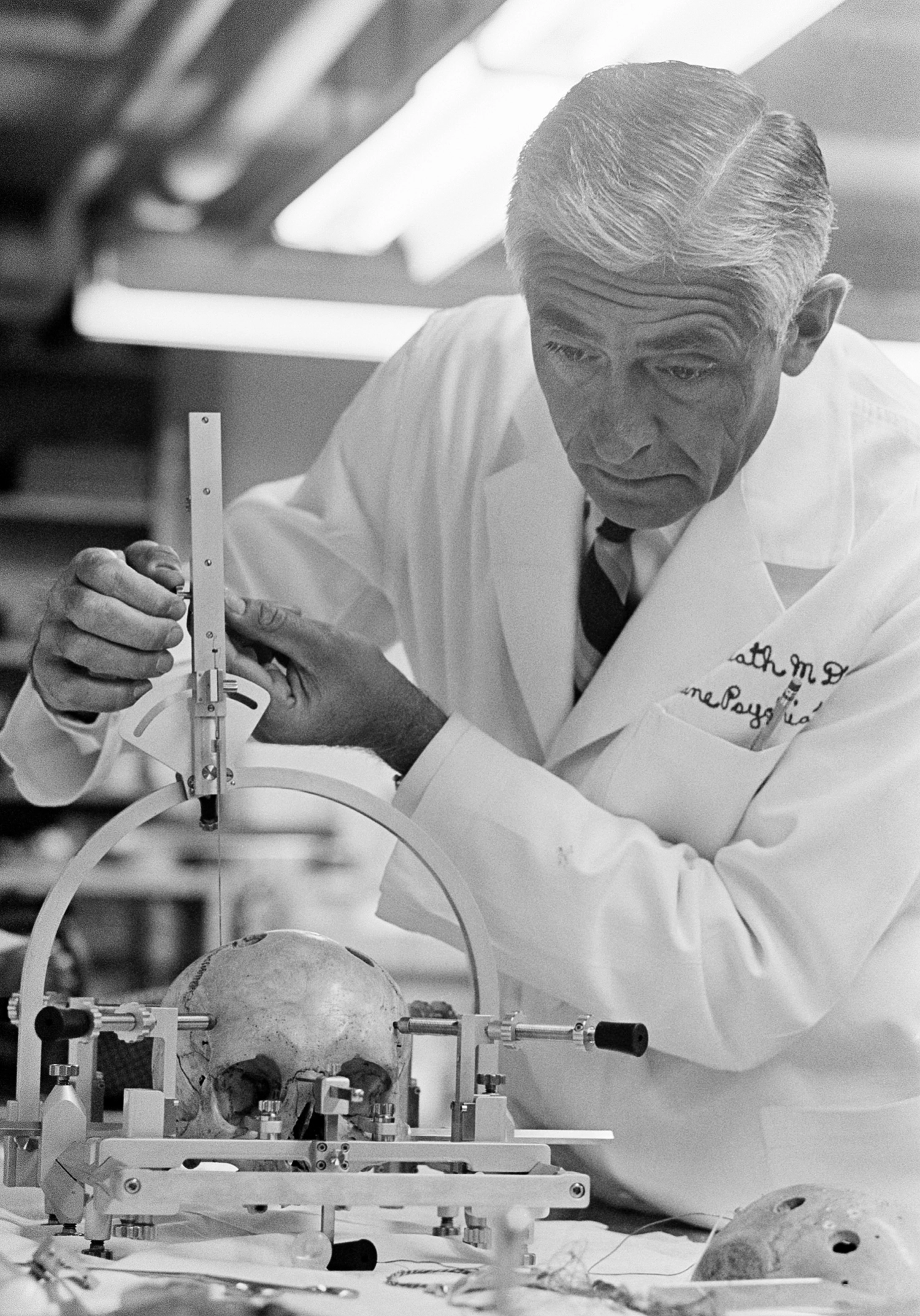
Robert G. Heath demonstrating deep-brain-stimulation electrode placement
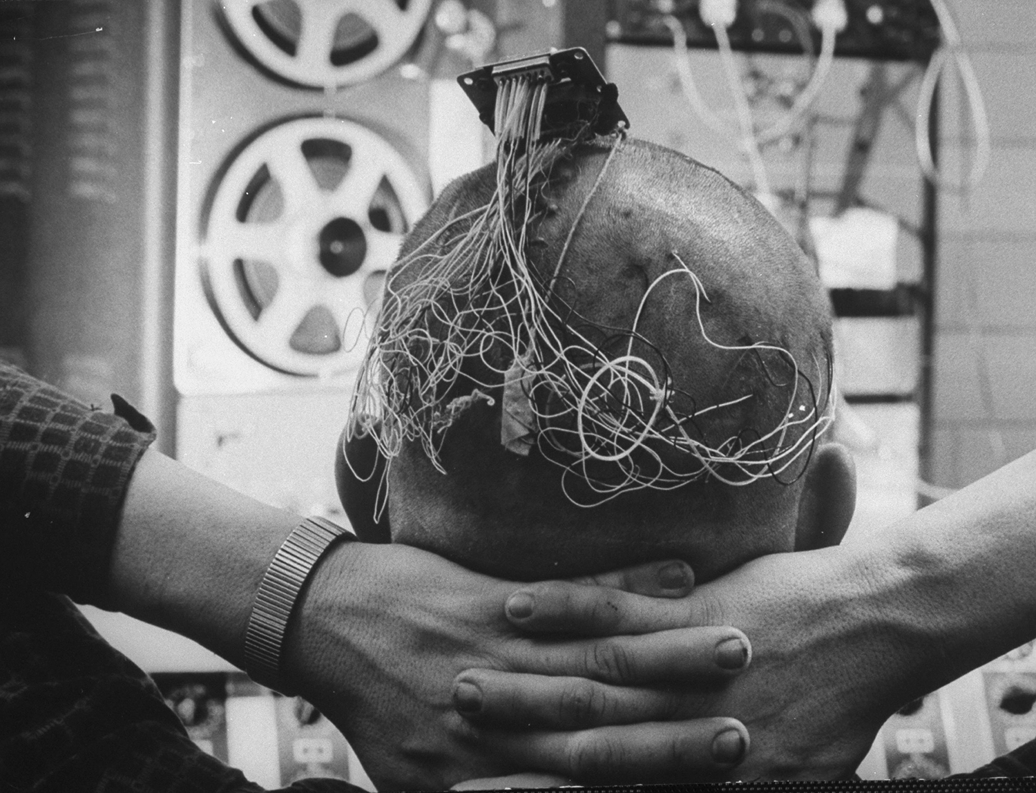
One of Heath’s patients with multiple electrodes implanted
On the other hand, when the dopamine-producing neurons of rats are destroyed, the rats become passive and starve to death, even if food is “literally under their noses.” 38 If food is placed into their mouths, they eat it with evident pleasure, but no matter how hungry they get, without dopamine, they aren’t spurred to action.
Now, put yourself back in the worm’s place. If you realize your prediction of future food is being violated by a decline in the ambient food near your head, you will want to turn. The turn, even if random (as with a bacterial tumble), will reorient you toward a direction where the food level might once again go up—and if that doesn’t work, just keep turning until it does. In an area of peak food, every direction leads to a decline, so the animal will continue turning (or tumbling) in place, which is, as it happens, the optimal food-exploitation strategy.
Serotonin neurons serve the converse function. They sense food in the animal’s throat rather than in the environment. As serotonin builds up over time, the message becomes: “enough, I’m satiated.” The effect of dopamine will be quelled, along with the impulse to move at all. Postprandial torpor will set in, the better to digest.
Thus, we can crudely characterize dopamine and serotonin as the chemicals associated with “wanting” (dopamine) and “getting” (serotonin). The word “crudely” is important to emphasize here, though. Both serotonin and dopamine serve complex and only partly understood functions in animals with big brains. 39 Decreased dopamine levels, for instance, have not only been implicated in “not wanting,” but also in lack of “vigor,” or drive to exert effort for a reward—which isn’t quite the same. Are hungry, dopamine-deprived rats not eating due to a lack of desire, a lack of vigor, or both? These remain open questions. 40
In early bilaterians, though, dopamine and serotonin affected behavior more straightforwardly, by providing smoothed averages, accessible to other neurons, approximating food expected and food eaten. Neurons that were not in direct contact with either the outside world or the throat could then modulate signals sent to the muscles appropriately.
This developmental stage appears to be preserved in Acoela, an ancient order of small marine worms that diverged from other animals more than 550 million years ago. With simple body plans, Acoela have no gut and no circulatory or respiratory systems. They move (either swimming or crawling between sand grains on the sea bottom) by means of “cilia,” little hair-like projections covering their exterior, whose movements are locally controlled.
In addition to a distributed nerve net, Acoela have a sort of “brain cap,” an aggregation of neurons at the front end, coinciding with sensors, including a simple eye. 41 They can use complex repertoires of sensory-guided behavior to actively hunt, modulated by dopamine and serotonin. 42 Yet the “brain” seems not to be highly organized. If one of these worms is cut in half, then, like the neurally decentralized Hydra, each half can regenerate into a whole animal. Signaling molecules exchanged among the muscle cells appear to orchestrate the patterning and re-generation process. 43
If the tail of an acoel is cut off, the front part of the animal regenerates a new tail, while the tail regenerates two heads, which subsequently divide into two new acoels
Bootstrapping
Animals with simple distributed nerve nets, like Hydra, show little evidence of learning in any form that a behavioral experimentalist would recognize, though every cell does continually regulate its own biophysics to ensure that it remains responsive to whatever signals it receives—a form of local learning. 44 This is consistent with the idea that these earliest nerve nets serve only secondarily for sensing the environment, having first evolved to help muscles coordinate coherent movement.
Rudimentary behavioral learning arises the moment anything like a brain appears, because, at this point, neurons in the head must begin jointly adapting to changing conditions in the outside world. Every connection or potential connection between one neuron and another offers a parameter—a degree of coupling—that can be modulated to suit the circumstances, even if the “wiring diagram” is genetically preprogrammed or random.
To see why, let’s take the neuron’s point of view, and imagine that it is simply trying to do the same thing any living thing does: predict and bring about its own continued existence. 45 Some aspects of this prediction will certainly have been built in by evolution. For example, if dopamine is a proxy for food nearby, the neuron will try to predict (and thereby bring about) the presence of dopamine, because prolonged absence of dopamine implies that the whole animal will starve—bringing an end to this one neuron, along with all of its cellular clones. Even a humble cell has plenty of needs and wants beyond food, but without food, there is no future.
Therefore, if the neuron is not itself dopamine-emitting, but its activity somehow influences dopamine in the future, it will try to activate at times that increase future dopamine. Aside from neuromodulators like dopamine, the neuron’s inputs come either from other neurons or, if it’s a sensory neuron, from an external source, such as light or taste. It can activate spontaneously, or in response to any combination of these inputs, depending on its internal parameters and degree of coupling with neighboring neurons. Presumably, at least one of its goals thus becomes fiddling with its parameters such that, when the neuron fires, future dopamine is maximized.
I’ve just described a basic reinforcement learning algorithm, where dopamine is the reward signal. As brains became more complicated, though, they began to build more sophisticated models of future reward, and, accordingly, in vertebrates, dopamine appears to have been repurposed to power something approximating a more sophisticated reinforcement learning algorithm: “temporal difference” or “TD” learning.
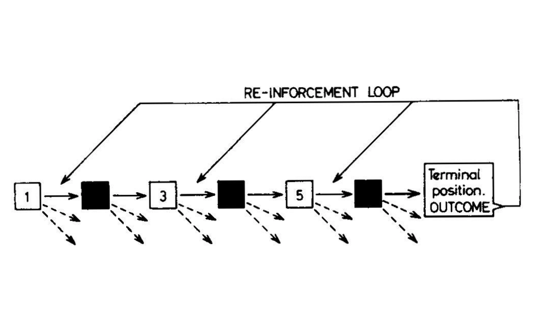
In 1961, AI researcher Donald Michie devised MENACE, the Matchbox Educable Noughts and Crosses Engine, an early reinforcement-learning algorithm for playing tic-tac-toe. Initially, lacking access to a computer, Michie implemented the algorithm using an array of 304 matchboxes representing unique board states, each containing beads representing the current best policy; Michie 1963.
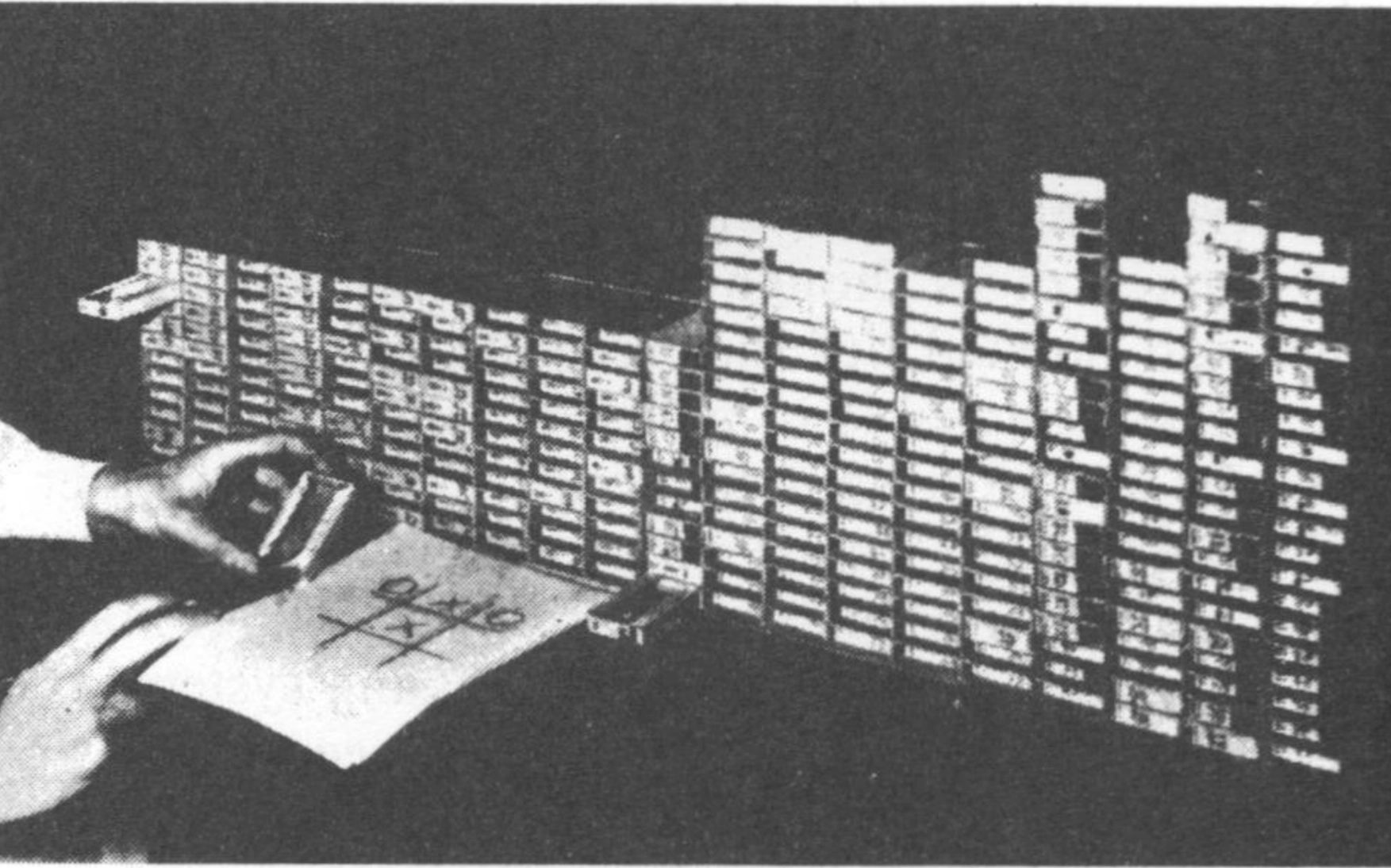
In 1961, AI researcher Donald Michie devised MENACE, the Matchbox Educable Noughts and Crosses Engine, an early reinforcement-learning algorithm for playing tic-tac-toe. Initially, lacking access to a computer, Michie implemented the algorithm using an array of 304 matchboxes representing unique board states, each containing beads representing the current best policy; Michie 1963.

In 1961, AI researcher Donald Michie devised MENACE, the Matchbox Educable Noughts and Crosses Engine, an early reinforcement-learning algorithm for playing tic-tac-toe. Initially, lacking access to a computer, Michie implemented the algorithm using an array of 304 matchboxes representing unique board states, each containing beads representing the current best policy; Michie 1963.
TD learning works by continually predicting expected reward and updating this predictive model based on actual reward. The method was invented (or, arguably, discovered) by Richard Sutton while he was still a grad student working toward his PhD in psychology at UMass Amherst in the 1980s. Sutton aimed to turn existing mathematical models of Pavlovian conditioning 46 into a machine-learning algorithm. The problem was, as he put it, that of “learning to predict, that is, of using past experience with an incompletely known system to predict its future behavior.” 47
In standard reinforcement learning, such predictions are goal-directed. The point is to reap a reward—like getting food or winning a board game. However, the “credit assignment problem” makes this difficult: a long chain of actions and observations might lead to the ultimate reward, but creating a direct association between action and reward can only enable an agent to learn the last step in this chain.
As Sutton put it, “whereas conventional prediction-learning methods assign credit by means of the difference between predicted and actual outcomes, [TD learning] methods assign credit by means of the difference between temporally successive predictions.” 48 By using the change in estimated future reward as a learning signal, it becomes possible to say whether a given action is good (hence should be reinforced) or bad (hence should be penalized) before the game is lost or won, or the food is eaten.
This may sound circular, since if we already had an accurate model of the expected reward for every action, we wouldn’t need to learn anything further; why not just take the action with the highest expected reward? As in many statistical algorithms, though, by separating the problem into alternating steps based on distinct models, it’s possible for these models to take turns improving each other, an approach known as “bootstrapping”—after that old saying about the impossibility of lifting oneself up by one’s own bootstraps. Here, though, it is possible.
In the TD learning context the two models are often described as the “actor” and the “critic”; in modern implementations, the actor’s model is called a “policy function” and the critic’s model, for estimating expected reward, is the “value function.” These functions are usually implemented using neural nets. The critic learns by comparing its predictions with actual rewards, which are obtained by performing the moves dictated by the actor, while the actor improves by learning how to perform moves that maximize expected reward according to the critic.
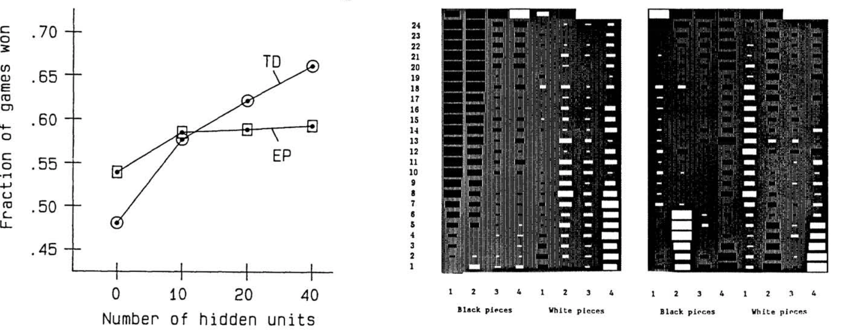
Gerald Tesauro’s TD-Gammon, an application of temporal difference reinforcement learning to backgammon, was able to beat expert human players more than half the time when the trained neural net contained more than ten hidden units (or neurons); Tesauro 1991.
A TD learning system eventually figures out how to perform well, even if both the actor and critic are initially entirely naïve, making random decisions—provided that the problem isn’t too hard, and that random moves occasionally produce a reward. Hence an experiment in the 1990s applying TD learning to backgammon worked beautifully, 49 although applying the same method to complex games failed, at least initially.
Beyond Reward
Around the same time, at the University of Fribourg’s Institute of Physiology, Wolfram Schultz’s lab had been studying the relationship between motor function and Parkinson’s disease, which was known to compromise movement via dopamine depletion. 50 In a typical experiment, Schultz and colleagues would record from single dopamine-releasing neurons in the brains of macaques while they performed simple motor tasks, which they needed to learn via Pavlovian conditioning. 51 A thirsty monkey, for instance, might need to learn which of two levers to pull in response to a flashing light to get a sip of juice. The researchers made the following observations:
- Dopamine neurons normally spike at a moderate background rate.
- When the monkeys first stumbled upon an action producing the sugary drink, the spiking rate of these dopamine neurons rose.
- Once the monkeys figured out the association between the visual cue and the reward, extra dopamine was no longer released when the treat came, but was released earlier, when the visual cue was presented. This coincided with the monkeys licking their lips, akin to the salivation of Pavlov’s dogs.
- If, following the visual cue, the treat was withheld, then activity of the dopamine neurons subsequently decreased—that is, they went quiet relative to their background rate.
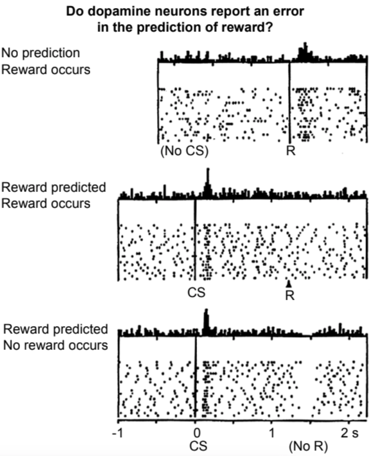
Recordings from a dopamine neuron when an unexpected reward is received, an expected reward is received, and an expected reward is not received; Schultz, Dayan, and Montague 1997.
When Peter Dayan and Read Montague, then postdocs in Terry Sejnowski’s lab at the Salk Institute in San Diego, saw these results from Schultz’s group, they realized that dopamine was acting precisely like a temporal-difference learning signal. 52 This is the signal whereby the brain’s “critic” tells the “actor”: please reinforce whatever behavior you’re doing now, because I predict it will lead to a future reward. Long sequences of actions that ultimately lead to a reward can be learned this way, with the TD learning signal shifting earlier and earlier in the sequence as the learning progresses.
The repurposing of dopamine from a simple reward signal to something like a temporal-difference reinforcement-learning signal might follow naturally from the growth of brain structures both “upstream” and “downstream” of the dopamine-releasing neurons. Remember that even among the earliest bilaterians, dopamine no longer represents food, but nearby food. In this sense, dopamine is already a prediction of food, not a food reward in itself. Predicting dopamine is thus a prediction of a prediction of food.
A predictive symbiosis between neural areas upstream and downstream of dopamine will therefore result in the upstream areas being able to make higher-order predictions (hence longer-range forecasts), thus acting as an increasingly sophisticated critic or value function. Meanwhile, the downstream parts become an increasingly sophisticated actor, or policy function, smart enough to learn how to make better moves using these longer-range forecasts.
This may help to explain the approximate fit between the TD learning paradigm and at least one major role played by dopamine in the brains of vertebrates. 53 Like many primal feelings, “something good is within reach” is a simple, useful signal that a worm can infer directly from smell, and a larger-brained animal like us can infer through a much more complex cognitive process. That is a useful signal for many parts of the brain, since they are all invested in producing good outcomes for the organism as a whole; hence dopamine signaling has been conserved for hundreds of millions of years, and its role has remained, if not the same, at least recognizable throughout those eons.
Still, we should be careful not to interpret these experimental findings about dopamine as proof that the brain implements TD learning as Sutton formulated. That can’t be the whole story. For one, we have ample evidence that humans, and likely many other animals, are even more powerful learners than the TD algorithm is. Advanced board games we have no trouble playing, for instance, are beyond the reach of TD learning. Additionally, as I hinted earlier, recent experiments suggest that dopamine encodes information well beyond that of a TD error signal. 54
None of this should surprise us. Brain regions that symbiotically predict their environment and each other are not restricted to implementing simple learning algorithms, or communicating using cleanly definable mathematical variables, any more than human emotional expression is limited to a single dimension or natural language is restricted to logical grammar. Like every other approach to machine learning described in this book, TD learning is an elegant conceptual simplification that sheds light, but does not illuminate every corner. It is neither a complete nor an exact representation of what the brain does.
In 2016, DeepMind’s AlphaGo model made headlines by achieving a major milestone in AI history. This program, based on a more elaborate descendant of TD learning (which we’ll explore in chapter 5), defeated reigning Go champion Lee Sedol in four out of five games. 55 The news came amid reports of machine learning besting humans at a rapidly lengthening list of tasks previously considered “safely” beyond AI’s capabilities. 56
Lee Sedol reacting to AlphaGo’s move 37 during the second game of their five-game match in Seoul on 10 March 2016; Kohs 2017.
Despite this impressive showing, neurophilosopher Patricia Churchland pointed out fundamental limitations in the AI paradigm at the time relative to what real organisms with real brains do. In response to AlphaGo’s victory, Churchland wrote an essay entitled “Motivations and Drives are Computationally Messy,” 57 noting:
The success of [artificial neural nets like AlphaGo] notwithstanding [ … their] behavior is a far cry from what a rat or a human can do […]. Maintaining homeostasis often involves competing values and competing opportunities, as well as trade-offs and priorities[…]: should I mate or hide from a predator, should I eat or mate, should I fight or flee or hide, should I back down in this fight or soldier on […]. The underlying neural circuitry for essentially all of these decisions is understood if at all, then only in the barest outline. And they do involve some sense of “self” […].
It’s true. A pure reinforcement-learning approach, no matter how fancy the algorithm, cannot account for realistic animal behavior, because real animals—including us—are not optimizing for any one thing (except, maybe, when we’re playing championship-level Go). However, “real AI” may be simpler than Churchland—or any of us—imagined in 2016.
Close mathematical relationships exist among the various known machine-learning methods, 58 and ongoing theoretical work will likely unify them further. While this remains an active research area, I believe that a unified theory of learning will ultimately encompass evolution, brains, and, as special cases, established ML methods. Such a unification would:
- Frame the central problem as active prediction of the future given the past;
- Not distinguish between learning and evaluation or inference, but instead recognize that prediction must occur over all timescales; 59
- Synthesize prediction with an extended theory of thermodynamics in the spirit of dynamic stability, as sketched for bacteria in chapter 2; 60 and
- Explain how mutual prediction between agents can lead to collective, nonzero-sum outcomes.
A unified theory would illuminate the deep relationships between computing, machine learning, neuroscience, evolution, and thermodynamics. Such a theory is still incomplete, but this book offers a glimpse of what it may look like, predicated on a hypothesis about what nature does at every scale, from cells (and below) to societies: unsupervised sequence prediction.
Predicted sequences involve continued existence. If they did not, then the organisms that made those (self-sabotaging) predictions wouldn’t still be here. Moreover, as we’ll soon explore, when entities that can sense each other begin to mutually predict each other, it becomes easy for them to enter into a symbiotic partnership in which their joint future existence is more secure than their individual existences.
Let’s call this view “dynamically stable symbiotic prediction.” What would it imply about the brain? Unlike TD learning or any form of pure reinforcement learning, symbiotic prediction does not imply that animals optimize any single reward, whether food or dopamine. On the contrary, such single-mindedness would not be conducive to either mutualism or survival in the real world, hence it would not be dynamically stable. Per Churchland, “Maintaining homeostasis often involves competing values and competing opportunities, as well as trade-offs and priorities.” This is even truer in social settings. There are many ways to be alive in this world, but all of them must involve continuing to exist in the future, and existence requires ongoing relationships.
Let’s pull these threads together and summarize: as evolution built on the design of simple Acoela-like bilaterians, additional neurons appeared in heads. This happened because neurons are themselves replicators, and, like all replicators, they will colonize any favorable niche, 61 in particular when that neural proliferation symbiotically helps the whole organism. Once this brain-knot began to grow, more complex neural networks developed, capable of handling more sophisticated sensory modalities, like hearing and camera-style vision. With help from neuromodulatory signals like dopamine, such brains were also able to predict increasingly subtle patterns relevant to the whole organism over ever-longer timescales.
Thus animals acquired the computational power to develop behaviorally relevant models of other complex animals, resulting in the kinds of early “social intelligence explosions” evident in the Cambrian period.
In 2017, during the heyday of convolutional neural nets, an episode of the painfully accurate Silicon Valley TV comedy aired that involved a “Not Hotdog app,” which was entirely equivalent to my scenario here; Seppala 2017 ↩. I’m just going for a healthier menu.
In math: the banana neuron’s activation is the dot product of its input weight vector with the embedding vector.
With the softmax function, this invariance is only approximate; changing the embedding layer’s banananess will still slightly affect the output. This feature is essential for backpropagation to work; the neural net can’t be learned if there’s no way to tell whether a tweak in the weights is making the output better or worse.
In math, applying a sequence of linear transformations is equivalent to applying a single linear transformation: A(Bx)=(AB)x. Even so, “deep linear networks” can be theoretically interesting, especially for studying the dynamics of learning. Saxe, McClelland, and Ganguli 2013; Q. Li and Sompolinsky 2021 ↩, ↩.
This theoretical result holds for nearly any kind of nonlinearity, though some nonlinearities are much better than others in practice. A great deal of work over the years has gone into designing nonlinearities that are fast to compute, efficient for learning, and don’t “blow up” numerically.
The “pretty much” is here because technically, linear transformations include both rotation and scaling.
Technical note: the dimensionality reduction approach Refik used was “t-distributed stochastic neighbor embedding” (t-SNE), which is a highly nonlinear operation designed for visualization rather than analysis. Thus linear (or planar, or hyperplanar) separation afterward typically won’t work, though the bananas will likely end up clustered together.
Tan et al. 2018 ↩.
This neglects the slight change we would also make to turn the “not banana” neuron into a “neither banana nor apple” neuron, but that’s a minor detail.
Qi, Brown, and Lowe 2017 ↩.
Tanaka and Pierce 2009 ↩.
Kohl 1993 ↩. The effect likely does not depend on infants forming discrete sound categories from the start, as Kohl believed, but rather learning the invariant embeddings that represent their speech environment; Feldman et al. 2021 ↩.
In more precise mathematical language, they show that while the specific weights of a given network are determined by their random initialization, these weights are only unique up to an arbitrary rotation in the high-dimensional space of per-layer weights; see Guth et al. 2023; Guth and Ménard 2024 ↩, ↩.
Some details are glossed over in this brief description; see He et al. 2021 ↩.
Inexplicably, our retinas are wired back to front, with the plumbing in front of the photoreceptors—nearly a proof of lack of intelligent design. Octopus retinas, which evolved independently, are wired the right way round, with the light sensors in front.
These experiments are reviewed in Churchland, Ramachandran, and Sejnowski 1994 ↩.
Such recordings are rare; they are made when neurosurgeons are trying to figure out how best to operate on someone’s brain when they need to, while sparing as much function as possible. Researchers gather precious human data of this kind when they can, but any scientific aims are always secondary to clinical aims.
Hunter, Spracklen, and Ahmad 2022 ↩.
Qiu, Huang, and Fu 2023 ↩.
Gross 2002 ↩.
Quiroga et al. 2005 ↩.
Jennifer Aniston and Brad Pitt were married from 2000–2005, so this neuron might have needed to find a new gig after they split.
This is 128 × 127 × 126 × 125 × 124 × 123 × 122 × 121 × 120 × 119 × 118 × 117 × 116 × 115 × 114 × 113.
Historically, these terms were used in fencing: whoever is thrusting is the agent, and whoever is receiving or suffering the blow is the patient. In the history of medicine, similarly, the “patient” suffers passively while the surgeon or physician lances boils, cuts for stone, saws off limbs, punctures veins for bloodletting, and conducts other such swashbuckling maneuvers.
This also illustrates why the concept of multiple realizability only makes sense when there is a final cause.
In most cases there’s at least one synapse en route, but let’s not sweat the anatomical details.
Strogatz 2004 ↩.
Sarfati et al. 2022 ↩.
Burkhardt et al. 2023 ↩.
Godfrey-Smith 2024 ↩.
Goulty et al. 2023 ↩.
Heath 1963 ↩.
Berridge and Robinson 1998 ↩.
Gershman et al. 2024 ↩.
Zénon, Devesse, and Olivier 2016 ↩.
Achatz et al. 2013 ↩.
They also engage in “penis fencing.” Google it if you’re feeling brave.
Raz et al. 2017 ↩.
Local adaptation also results in weak forms of learning known as “sensitization” and “habituation.” Cheng 2021 ↩.
Relatedly, J. J. Moore et al. 2024 ↩ suggest that single neurons can act as optimal feedback controllers.
R. R. Bush and Mosteller 1951; Rescorla and Wagner 1972 ↩, ↩.
Sutton 1988 ↩.
Sutton 1988 ↩, emphasis mine.
For a comprehensive historical overview of the development of TD learning and its convergence with dopamine research, see Colombo 2014 ↩.
Romo and Schultz 1990 ↩.
Montague, Dayan, and Sejnowski 1996 ↩.
The original experiments were done with primates, but evidence suggests that dopamine plays a similar role, mediated by the same brain structures, in all vertebrates. Analogous systems involving related neuromodulatory chemicals appear to have evolved in invertebrates too. Mizunami and Matsumoto 2017 ↩.
Fouragnan, Retzler, and Philiastides 2018; Diederen and Fletcher 2021 ↩, ↩.
C.-S. Lee et al. 2016 ↩.
Shoham et al. 2017 ↩.
Churchland 2016 ↩.
For instance, Sutton 1988 ↩ describes how TD learning and supervised learning can both be understood as gradient descent methods for sequence prediction.
Today’s separate treatment of inference (typically involving short timescales), so-called “adaptation” (intermediate timescales), and learning (long timescales) is an artifact of the cybernetic formalism described in “Negative Feedback,” chapter 3.
See “Complexification,” chapter 1.