Being in Time
I hope I have now convinced you that life is inherently computational, though we’ve only scratched the surface of what it actually computes. The minimal functionality for a dynamically stable life form is, of course, replication, or, more precisely, self-construction. Open-ended evolution requires a von Neumann constructor, which is necessarily also a full-fledged Turing machine. The constructor makes it possible to build complex and recursive structures like a tree’s branches or an animal’s circulatory system.
But the environments in which construction and replication take place look nothing like the pristine grid worlds of von Neumann’s cellular automata. The real world is messy, ever-changing, intrusive. To maintain any kind of integrity in such a world, a computational system needs a protective boundary. 1 Yet the boundary can’t be absolute, because life can never be self-sufficient: computation requires energy, and self-construction requires matter.
Outputs are necessary, too, because neither computation nor growth can be perfectly efficient. Computation generates heat, which has to go somewhere. And not every atom that enters a living system can become a functional part of it. Since matter and energy can’t be created or destroyed, an organism must therefore shed matter (excretion) and energy (waste heat). Like a vortex, life is a dynamical pattern that can only exist in the flux of a larger environment.
The sort of computation we call “intelligence” thus arises because of this need for life to interact with its surroundings. Those surroundings invariably include other life forms, opening the door to higher levels of symbiosis, as will be discussed later in the book. Here, though, we’ll explore intelligence at its most basic: in single-player mode.
Imagine a simple, single-celled life form—say, a bacterium. Its cell membrane separates a “self,” on the inside, from the outside world. But, as mentioned, the separation can’t be total. Studded with pores and ion pumps, able to ingest nutrients and excrete wastes, cellular membranes are selectively permeable to matter and energy—just like our bodies.
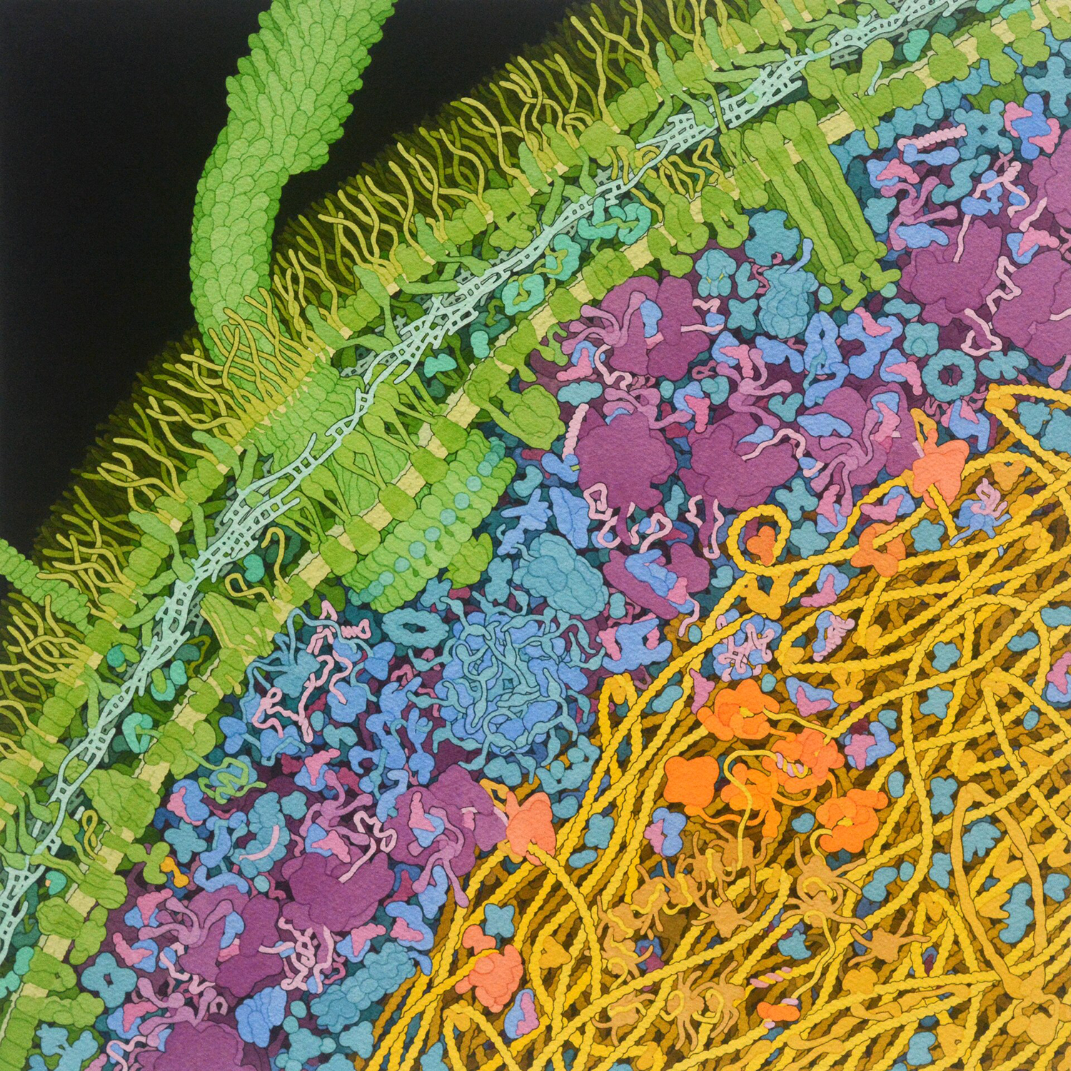
Illustration of the molecular machinery inside an E. coli bacterium by David S. Goodsell, RCSB Protein Data Bank, 2021
That also makes them permeable to information, because matter and energy aren’t generic. A potassium ion isn’t interchangeable with a calcium ion, and a red photon isn’t the same as an ultraviolet one. These inputs will have different effects on the organism. Thus, every input is also, necessarily, a kind of sensor. Given the value of sensory information for an organism’s survival, some inputs have evolved to be primarily informational. A receptor may “taste” a molecule without actually pulling it through the membrane, for example. The point is to gather information.
To process that information, a bacterium has something like a “brain.” 2 It consists of a dynamical network of interacting genes and proteins that are both affected by sensory data and can control cellular processes and behaviors. This biochemical “brain” also receives inputs from within the cell, such as metabolic status and available energy, allowing internal states like “hunger” to modulate behavior.
Some bacteria can swim, using a corkscrew-like bundle of motorized filaments called a “flagellum”—though steering, in the usual sense, is impossible. Due to the simplicity of the bacterial body plan, the irrelevance of gravity, and the molecular buffeting that characterizes life in water at such small scales, the cell can’t distinguish left from right, or up from down. When swimming, it can only “run,” rotating its flagella clockwise to propel itself forward, or “tumble,” running some of its flagellar motors in reverse and causing the cell as a whole to spin chaotically, randomizing its orientation.
A classic series of studies by biophysicist Howard Berg and colleagues in the 1970s shows how, simply by tumbling more often when food concentration is dropping and less often when it’s rising, bacteria on average swim toward places with higher food concentration—a behavior known as “chemotaxis.” 3 They can use the same approach to swim toward warmth (“thermotaxis”) or, for photosensitive bacteria, toward light (“phototaxis”).
Chemotactic E. coli bacteria swimming toward a sugar crystal
Not that a bacterium can directly measure concentration, temperature, or light level, let alone differences in these properties along its microscopic body length. It’s just too small. Relative to every relevant feature of the world it lives in, the bacterium is point-like; one could almost say that it exists only in time, not in space. That is, it experiences life as a sequence of events, and anything it might learn or observe about its spatial environment can only be inferred from that event sequence.
These events are all discrete, or “digital,” even when they relate to continuous physical quantities, such as chemical concentration—because at bacterial scale, chemicals are only sensed one molecule at a time, as they dock and undock with receptors on the cell membrane. Photon absorption and temperature-dependent chemical events are quantized too.
While these discrete events are individually random, the ambient concentration, temperature, or illumination determine the rate at which they occur. Hence, a nominally continuous variable like concentration can only be estimated by counting such molecular docking events within a time window, effectively calculating a moving average. If the bacterium is swimming, and concentration varies over space, then a statistical tradeoff must be made in the estimation process. Counting for longer allows concentration to be estimated more accurately, but at the cost of washing out changes over time (or equivalently, over space). Bacteria are smart about this tradeoff, adapting their concentration estimation strategy to the situation. 4
Let’s explore how the estimation process works in more detail.
Batting Average
From a bacterium’s perspective, chemical concentration is a running estimate of the likelihood of future encounters with a molecule given a history of past encounters with it. In more technical language, if we call the sequence of molecular encounter events X, then the concentration is a time-varying estimate of the probability of X, which can be written as P(X).
If this mathematical notation takes you out of your comfort zone, let me try to make it up to you by offering an analogous situation from outside mine: baseball.

Aaron with the Milwaukee Braves in 1960
Here’s my naïve understanding of the most famous statistic in sports, the batting average. Every time a baseball player is at the plate, they may either succeed, which we could represent as a one, or fail, which we could represent as a zero. Success often involves hitting the ball, but apparently certain ways of hitting it don’t count, and other apparent failures, such as the “sacrifice fly,” are actually not? (If I hadn’t furtively brought a sci-fi novel to the one baseball game my American relatives dragged me to when we moved to the US, I might have learned these things earlier.) Anyway … over time, a player’s batting history can be represented as a string of ones and zeros, with a single bit produced every time they’re at bat. The proportion of ones—in other words, the average value of all those ones and zeroes—is a player’s batting average.
We can study the data more closely, because baseball nerds have put the complete batting histories of Major League Baseball (MLB) players online, going back many decades.
Consider Henry “Hank” Aaron, widely held to be one of the greatest players of all time. During a long career in the Major Leagues, from 1954 to 1976, Aaron stepped up to the plate over twelve thousand times, and 30.5% of the time, he successfully hit the ball and got on base, or better. This “.305” average is considered awesome.
No player’s performance is constant over time, though. It’s easy to see this by calculating batting averages for individual seasons (spanning six months every year, from April through September). Now, we can see that over the first few years of Aaron’s career, his batting average went up, peaking at over .350 in 1959. Like anything else, baseball has a learning curve.
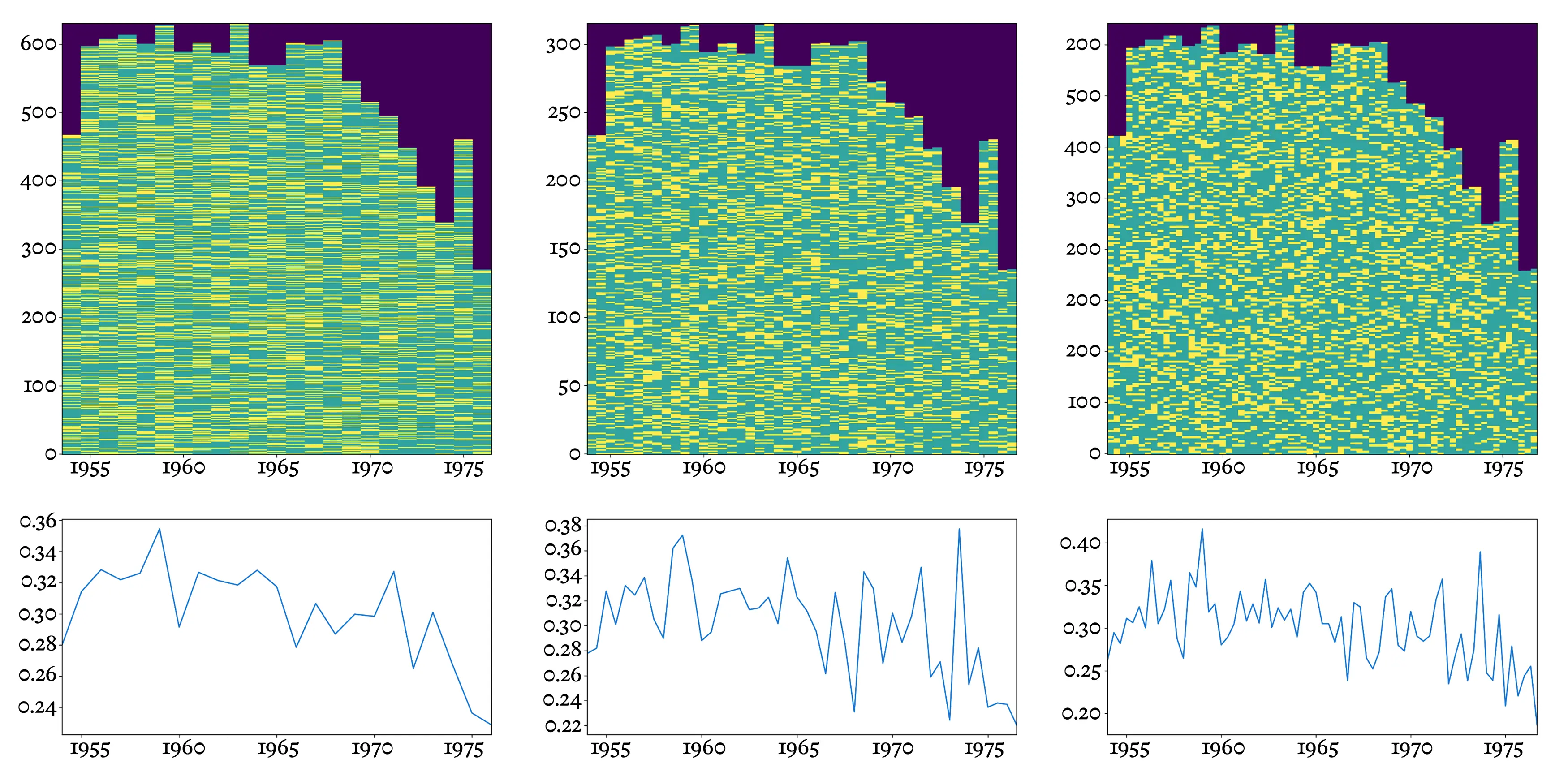
Hank Aaron’s complete batting history (top row), and batting averages (bottom row), broken down into 6-month windows covering a complete yearly baseball season (left column), 3-month windows (middle column), and 2-month windows (right column).
But alas, bodies age, and small injuries accumulate. His performance declined, first gradually, then more sharply; by the end of his career he was batting below .250. By that point he was going up to bat only half as often—no doubt, because the manager was keeping a close eye on batting averages, and as Aaron’s declined, he was increasingly sidelined.
We’ve gone from considering career averages to six-month season averages, but nothing prevents us from averaging over shorter windows—three months, two months, or even single months. This finer-grained analysis brings new information into view, up to a point. Using three-month windows, we can see that Aaron reached his career peak just a few years before retiring, averaging an amazing .378 between July and September of 1973. (He finished that year with 713 home runs, just one behind the world record set in 1935 by Babe Ruth. Thousands of letters to Aaron poured in, some from fans, others filled with hate and death threats, from those appalled at the prospect of a Black man breaking baseball’s most sacred record.)
Still, over time, not only had Aaron’s season average declined; his performance had also become more uneven. So while the highs remained high, they were interspersed with lower and more unpredictable lows. Hence a short averaging window that would have been highly predictive early in Aaron’s career would have shed less light on the future later on.
Part of the effect is simply due to lack of data. When we average over shorter intervals, or Aaron goes to bat less often, the estimate becomes noisier because there are fewer bits to average. In the limit, if our window shrank all the way to a single at-bat, the “average” could only assume two values, 0.000 or 1.000, making it useless as a predictor of future performance. Clearly, then, there’s an ideal size of averaging window, large enough to accumulate decent statistics but small enough to register changes over time. The ideal window size will depend not only on the rate of at-bats, but also on how often a hit occurs and on how consistent the player is.
All of this is to say: if X is a sequence of discrete events in the past, whether hits for a baseball player or food-molecule encounters for a bacterium, P(X) smooths those discrete events into a continuously varying average rate using an appropriately sized averaging window—which is also an estimate of the likelihood of encountering such an event in the immediate future. Although this quantity is a description of the past, it’s a predictive model. If no events have occurred for a while, the likelihood is low; if a flurry of events just started, the likelihood is high; if the rate has been increasing, then a good estimate will be higher than the historical average, and if the rate has been decreasing, a good estimate will be lower. 5
So, are batting averages “real”? It’s obvious that Hank Aaron’s batting average wasn’t a measurement of some physical quantity out in the world, or in his body or mind—though neither was it unconstrained by the physics of balls and bats, the psychology of pitchers, or the physiology of aging bodies. It didn’t have any one true value, either, in that it could be estimated in many ways, and on many timescales—though some estimates are better than others, in the sense of being more predictive. Despite their fuzziness, though, batting averages matter to players, managers, and fans alike, because they both predict and affect the future.
The same applies to the kind of statistical measurements that matter to bacteria. Like billiard balls, molecules are discrete objects, subject to microscopic physical laws that don’t in any way involve or require macroscopic concepts like “concentration” or “temperature.” But if a bacterium needs to predict its likelihood of encountering food, it must estimate concentration based on recorded events, not unlike baseball hits.
As described in chapter 1, Boltzmann’s development of thermodynamics—the Ideal Gas Law, for instance—defines quantities like pressure, temperature, and concentration using mathematical models and approximations of the same kind. These, too, involve counting molecules or events within a time window or spatial box.
Instruments like thermometers or pH strips do the same using an experimental apparatus rather than theory. So does a digital camera, by counting the photons absorbed by each pixel. In short, just like batting averages, variables like brightness, temperature, pH, and concentration rely on models: ways of predicting future phenomena using past statistics.
(No) Things in Themselves
We can either conclude that properties like temperature are not “real”—a path that ultimately leads to the solipsistic denial that anything is “real”—or we can reappraise what it means for something to be real.
Outside pure math, “reality” can seldom be fully pinned down. We’ve seen how a concept like “temperature” falls apart when we ask about how hot or cold a medium is as its pressure or density drops toward zero, where averaging is no longer reliable. So, if we’re asked a question like “What is the temperature of outer space?” we should counter with more questions to answer meaningfully. Is this about calculating how hot a satellite’s solar panel will get? (Answer: it depends entirely on which way it’s pointed relative to the closest star, and on the shadows of any nearby moons or planets.) Is it about determining how comfortable your hand will feel if exposed to outer space? (Answer: don’t do it.) For a bacterium adapted to a watery medium, these simply aren’t relevant questions. One might as well ask a person, “How does a neutron star taste?”
Like taste, temperature is not a “thing in itself.” 6 It doesn’t pre-exist somehow in an unobserved universe. It is, rather, an observer-dependent model whose usefulness, from the observer’s viewpoint, depends on its behaviorally relevant predictive power. This is true not only of temperature, but of all the macroscopic phenomena we care about and describe using language, like “musical note,” “chair,” “bacterium,” or “person.”
It may even be true of phenomena like “an electron,” but here we run into limits in our understanding of the universe’s fundamental laws. “Electron” may merely be the name we assign to a certain kind of propagating disturbance in a quantum field, or it may have some more fundamentally “digital” nature that physicists investigating the subbasement of reality could one day discover. 7 And are quantum fields themselves “real”? Who knows?
Whether electrons, photons, quarks, and the various associated elementary forces are “real” and are observer-independent “things in themselves,” higher-order objects or features like temperature, pressure, chairs and tables, bacteria and people seem, at first blush, to be mere ideas, or “epiphenomena.” The unobserved universe doesn’t care about such ideas; after all, the continued existence of a chair doesn’t depend on whether someone is around to conceive of that bunch of atoms as “chair.” Atoms everywhere are governed by the unthinking laws of physics. 8
The mathematician John Conway’s “Game of Life” offers a useful illustration. It’s not really a game, in that there are no players, no score, no winning or losing. It’s just a set of rules that describe, given the state of the game board, what its next state will be. (This should sound familiar. Conway’s Life is, in fact, the most famous example of a cellular automaton, though von Neumann didn’t live to see it.)
Conway’s Game of Life in a toroidal world (i.e. the top edge connects to the bottom, and the left edge connects to the right), initialized with an arbitrary pattern
The rules are simple:
- Like pixels or graph paper, the world consists of a grid of square cells. 9
- Each cell can be “alive” or “dead.” We can visualize these states by coloring them black (alive) or white (dead).
- At every time step, the state of each cell is determined by the state of that cell and its eight neighbors during the previous time step.
- If the cell is alive, then it stays alive only if it has either two or three live neighbors.
- If the cell is dead, then it springs to life if it has exactly three live neighbors.
Under these rules, an entirely dead board will remain dead forever; that is a so-called “fixed point” or “steady-state solution.” As you can easily confirm with pen and paper, a 2×2 block of live cells on an otherwise dead board is also a steady state.
Conway and others have discovered that Life’s simple “physics” can produce many interesting higher-level phenomena, too. For instance, certain configurations of five live neighboring cells form a stable four-state cyclic pattern that appears to move diagonally through space, called a “glider.” A more complex configuration of cells forms a “glider gun,” in which a piston-like reciprocating mechanism pumps out an endless stream of gliders.
A glider gun in Conway’s Game of Life
In the Game of Life, one can build a lot of complex machines using a few simple ingredients like gliders and glider guns. In fact, it has been proven that, like von Neumann’s original cellular automata, Life is Turing complete; despite its simplicity, an enterprising engineer can create a general-purpose computer in Life. 10 (In a particularly striking feat of recursive nerddom, the computations required to simulate Life have even been programmed in Life! 11 This has to be seen to be believed.) It follows that the seemingly trivial universe of Life could carry out arbitrarily complex computations, including, perhaps, a simulation of our entire universe. 12
Life implemented in Life by Phillip Bradbury, 2012
Once a system can compute, its underlying physics become irrelevant to that computation—remember that, per Turing, all computers are equivalent. Therefore it’s just as valid to say that the computation doesn’t care about the physics as to say that the physics doesn’t care about the computation. This will matter to us later on, as it allows us to understand functionality in a living (or intelligent) system without needing to understand its underlying mechanism.
A die-hard physicist, though, can justifiably insist that neither gliders nor any of the infinitely complex things one can build in Life are “real” or “things in themselves,” in the sense that the rules of Life don’t involve any such objects. There are only dead and live cells, and the elementary rules for determining their next states. These facts, and these facts alone, comprise Life’s “Theory of Everything.” 13 Anything further is in the eye of the beholder.
As beholders, though, we can certainly see gliders. They appear to be real enough. What do we mean by this? We mean that, if we recognize a glider configuration, we can immediately predict what will happen next: it will cycle through four states and move diagonally until it encounters an obstacle. 14 If the glider were the only thing on an otherwise empty, infinite board, we could, with a single glance, predict every future state of the entire board, for all time. Compared to brute-force computation of the future state of every cell on the board, the effort saved is … well, infinite.
We could say, then, that gliders are real only and precisely because, as a concept or model, they are useful for predicting the future whenever the glider pattern arises. Recognizing and understanding gliders allows simulation without simulation.
Conway’s Game of Life with added “noise” from the microphone (try clapping)
Furthermore, the glider pattern is highly relevant in the Life universe, because the pattern is so simple that it tends to arise spontaneously. Meaning: if we imagine Life being played out on a large board where cells occasionally flip at random, gliders will form frequently. And when they do, we will immediately be able to predict their future trajectory—until and unless they are disrupted by noise, or by running into something.
Anthropic Principle
From a mathematician’s point of view, patterns like the glider and glider gun are special in that they correspond to “limit cycles”—generalizations of the idea of steady states (like the 2×2 block) to endlessly repeating loops of states. According to quantum field theory, the patterns we call “electrons,” “photons,” and “quarks” are much like gliders: stable (though oscillating) solutions to underlying field equations that don’t explicitly define such objects. This, too, should sound familiar: we’ve just encountered dynamic stability again.
Seen this way, gliders and elementary particles are simply the earliest steps in an evolutionary process, according to the maxim that whatever persists exists (and conversely, whatever is too dynamically unstable to persist … doesn’t).
Evolution doesn’t have to stop there. If eight gliders collide in just the right way, they will “react” to form a glider gun. 15 And not only is a glider gun stable; it also creates more gliders! Glider guns and a few other simple objects that can arise through glider collisions are the basic ingredients for building a Turing Machine.
Synthesis of a glider gun in Conway’s Game of Life out of eight gliders
Could Conway’s Life lead to abiogenesis, just as bff does? In our universe, that route involved primordial fields coalescing into elementary particles, electrons and protons coalescing into hydrogen atoms, the condensation of stars, the creation of increasingly heavy atoms through fusion, the formation of planets, and the subsequent events described at the beginning of chapter 1.
This may offer a solution to the age-old puzzle of why our universe seems to be so finely tuned for complex life to arise. As physicist Stephen Hawking wrote in A Brief History of Time, “The laws of science […] contain many fundamental numbers, like the size of the electric charge of the electron and the ratio of the masses of the proton and the electron. […] The remarkable fact is that the values of these numbers seem to have been very finely adjusted to make possible the development of life.” 16
For Hawking, and many others in the physics community, our very existence is thus evidence that many universes exist, for if there were only one, its compatibility with life would be a miracle … and physicists don’t believe in miracles. In a “multiverse” where the laws of physics vary between universes, the observation that our universe seems finely tuned to support our existence would simply be due to an observer bias known as the “anthropic principle”: of course the universe we happen to observe is finely tuned for life, because nobody could be around to observe the vastly greater number of sterile universes. It would be as absurd to claim that we’re “lucky” to live in this universe as it would be to claim that we’re lucky to live here on Earth and not on Mars, or inside the Sun, or in interstellar space—in short, in any of the vast number of places in the cosmos inhospitable to life.
This so-called “weak anthropic principle” is certainly correct. There are no poor “unlucky” people on Mars because no people are on Mars, period. It is, however, quite a leap to go from a puzzling observation about the life-friendly fine-tuning of physical laws to the “strong anthropic principle,” holding that any and all conceivable laws of physics must hold somewhere. Physicists should be uncomfortable with miracles, but many are equally uncomfortable with a multiverse where any and all laws exist. Is this really required to account for our own existence?
A more economical explanation is that the fundamental rules of our universe, like those of bff and Conway’s Life, allow for computation—evidently a much lower bar than allowing for life as we know it. 17 Multiple universes may or may not exist, but, either way, perhaps ours is not so special. Given a noise source, the simple logic of dynamic stability will select for stable entities, which can then start to combine into progressively higher-order dynamically stable entities: quarks into nucleons, electrons and nucleons into atoms, atoms into molecules, and so on. Entities like these can be understood as “proto-replicators,” subject to the tendency toward increasing complexification and computation described in chapter 1.
If the rules had been different, the “proto-replicators” would be different, and life’s software would have ended up on a different computational substrate. Perhaps quarks and electrons weren’t the only viable option. Indeed, even with the same rules, each evolutionary stage offers an expanding menu of possibilities. DNA isn’t the only possible information carrier, nor are amino acids the only possible “Lego bricks” for protein-like molecules. There’s certainly no reason all life on Earth should rely exclusively on right-handed sugars, as opposed to their mirror-image versions, the left-handed sugars. Regardless of such “just so” choices, the end result would be the same: replication, computation, and life.
Darwin may have been right in yet another way, then, when he wrote of abiogenesis that “one might as well think of origin of matter.” He was being facetious, but—why not? Matter might have evolved too.
The Umwelt Within
In describing Conway’s Life, we’ve allowed ourselves a third-person, God’s-eye view of a toy universe. But let’s now return to the bacterium living in our own world, pointlike relative to its vast watery environment, yet, on the inside, full of complex molecular machinery; technically brainless, but not unintelligent.
We’ve seen that the bacterial “brain” implements an adaptive algorithm for estimating chemical concentration as it swims, and it seems natural to call this measurement “purposive,” since it certainly looks like the goal is to eat and to avoid toxins—in short, to survive. I’ve argued that the very notion of “concentration” is something the bacterium appears to construct in the service of that purpose; chemical concentration is, to use pioneering biologist Jakob von Uexküll’s word, part of the bacterium’s umwelt: its “universe of the meaningful.” 18
Later, we’ll explore how the powerful social aspects of predictive models affect the future, but, for now, let’s stick to single-player mode. It’s not hard to see why a bacterium would care about its “batting average,” the rate at which it encounters molecules it can eat.
How much that rate can vary, and how low it can go, will of course depend on how depleted its reserves are. That’s why part of the bacterium’s umwelt is also its internal state; let’s call that state H, for “hidden.” In general, H includes a “comfort zone,” surrounded by a “danger zone”; beyond the danger zone lies death. In the simplest case, if we suppose that H represents the amount of available food inside the cell, estimating the “health-o-meter” P(H) will look like the same kind of smoothing process as that used to estimate P(X), but now based on discrete internal metabolic events H rather than measurements of the external environment X.
An organism’s “job #1” is to keep its internal estimate of P(H) in the comfort zone: this is “homeostasis.” The bacterium does this via actions, which we could also represent as a set of discrete motor events O (for “output”). These actions may be visible from outside—such as reversing the flagella to tumble—or they may be internal, such as turning on or off a gene or metabolic pathway. 19 Either way, homeostasis involves performing actions O given external observations X that maintain H within the comfort zone. This is intelligence in its most rudimentary form.
It’s common to suppose that something like “reinforcement learning” is at work here, allowing the organism to learn to perform any needed actions based on feedback that can be positive (“feeling more comfortable”) or negative (“feeling less comfortable”). However, the whole idea of grounding the emergence of intelligence in reinforcement learning—or supervised learning of any kind—implies an oracle that can administer rewards and punishments, or give correct answers. Where did this oracle come from? How did it become intelligent? Maybe there is no such oracle!
It’s simpler and more general to think about the evolution of intelligent behavior as arising from “unsupervised” learning (or, as it’s sometimes called now, self-supervised learning 20 ) of the combined or “joint” probability P(X,H,O). Bacterial populations that learn this joint probability distribution will not only “know” how to estimate nutrient concentration and their own internal state, but also, within some operating envelope, “know” what the consequences would be of acting in various ways under different internal and external circumstances. 21
Critically, this joint distribution is a prediction of self as well as environment—and of the consequences for oneself of various possible actions. The joint distribution includes all of the below “knowledge”:
- How to tell if you’re hungry;
- How to measure food concentration;
- How your next actions are likely to affect future food concentration; and
- How much less hungry you will be when you get that food.
Thus, the joint distribution contains everything one might want to “know” about how to behave to stay alive—at least, with respect to food. 22
Going forward, I’ll drop the scare quotes around “know” and “knowledge.” I’ve used quotes for two reasons. One reason is deep, and the other less so. The deep reason has to do with the distinction between a passive, abstract model and a real agent, whose predictions include actions that it takes and that determine the future. I’ll discuss this in more detail shortly.

Termite mounds along the old telegraph line on Cape York, Australia in 1983; the way termites build these impressive structures is often cited as an example of “competence without comprehension.”
But first, let’s dispense with the shallower reason for the scare quotes: the distinction many cognitive scientists draw between knowledge and competence. The phrase “competence without comprehension” has often been used to describe the way an agent can act as if it has knowledge without, apparently, having that knowledge. 23 Never mind bacteria; human baseball players or race-car drivers have amazing physical intuition in their domain of expertise, yet most baseball players wouldn’t be able to explain or reason about parabolic trajectories in general, and most race car drivers don’t know the equations for friction or centripetal force. So, do they “know” physics, or not?
This sounds like a more profound question than it really is. Math, physics, and, for that matter, the ability to explain things using language are all skills or competencies in their own right; none of them follows from learning how to swing bats, catch balls, or drive race cars—or vice versa. Plenty of nerds know physics well enough, but are so clueless about sports that they may need to look up what “batting average” means on Wikipedia. (Thank you, Wikipedia.) And of course symbolic math and language are far out of reach for an agent with the very limited computational capacity of a bacterium, even when such an agent’s learned competencies approach mathematical perfection in some practical domain.
As we’ll see when we explore large language models in chapter 8, symbolic skills and capabilities, like language and math, can also be fully represented as joint probability distributions—albeit enormous, complicated ones. Most of us who both know physics and have an intuitive understanding of how to drive or swing a bat don’t connect the two domains much, but, for some people, mathematical thinking and those physical intuitions might be closely associated, just as the sound of a voice and the motion of a speaker’s lips are; either way, it’s all in the big overall joint distribution P(X,H,O).
Latent Variables
Learning P(X,H,O) efficiently—that is, successfully representing it without exhaustively memorizing the probability of every individual combination of circumstance, state, and action—requires data compression. Without such compression, the size of the model, even for a simple organism like a bacterium, would be unwieldy; learning the model would therefore be very hard, and storing it or evaluating it would be expensive.
As we’ve seen, data compression involves finding patterns in data and factoring them out. For symbolic data, which are usually compressed “losslessly” by algorithms like those used for ZIPping files, such patterns generally take the form of repeated sequences. When the data are instead continuous and the compression is “lossy,” like that of MP3 audio or a JPEG image, finding those patterns allows irrelevant details to be ignored, exposing a smaller number of meaningful “latent variables.” 24
For the bacterium, the concentrations of molecules that bind to receptors are important latent variables. To see why, imagine the bacterium has one hundred receptors that bind to some chemical of interest, like aspartate (for E. coli, that’s a “yum”). Each receptor can be occupied or unoccupied by an aspartate molecule. Let’s suppose (I’m just making up numbers here) that occupancy is measured in millionths of a second, and the bacterium encounters between zero and a thousand aspartate molecules per second as it swims. Since the state of each receptor can be thought of as a binary digit, 0 for unoccupied and 1 for occupied, these hundred receptors produce a raw information stream that amounts to a hundred million bits of information per second. That’s a lot of bits per second, around ten times what it takes to transmit 4K video. 25
Luckily for a bacterium’s little brain, the overwhelming majority of this information is either useless or redundant. Since the cell is so small and there are no meaningful concentration differences along its length, it doesn’t matter which receptors are occupied—the receptors are “symmetric,” making any meaning extractable from them “invariant” to this symmetry. So we might as well just add all of these bits together.
Even when added up, the total is almost sure to be either 0 or 1 at any given time, because the occupancy time is short and the concentration is low. That means we’re already down to a mere one million bits per second. Then, when we consider that the exact timing of the docking events doesn’t matter—meaning that there is “local time symmetry,” or invariance to the precise timing of the docking events—we realize that we can just add up all of the ones each second, giving us concentration as an average occupancy rate over a one-second time window.
So, we’re back to averaging over a time window, as for calculating a batting average. That single number per second, which can be represented with only a few bits, accounts for the great majority of the real information coming in through those hundred receptors, though a little more information can be squeezed out by making the averaging window adaptive, as mentioned earlier.
Evolution will have honed in on something close to this compression scheme, because it sieves the useful information out and discards everything else. Such compression makes the overall distribution P(X,H,O) learnable, because the patterns relating X to H and O can only be generalized if the welter of irrelevant detail in X has been cleared away. In the language of information theory, the useful parts of X are the “signal,” while the discarded parts are the “noise.”
Remember, this signal is useful precisely because it’s a continuous estimate of the likelihood of a future docking event—though note that this continuous estimate is itself represented as discrete, stochastic signaling events within the cell, so in calling it a continuous number, we’re doing some modeling of the model. But we’re getting ahead of ourselves. More importantly, we’ve arrived at a practical definition of chemical concentration simply by thinking about what is relevant to the bacterium’s future given its past. Concentration is real because it’s predictive, just as the temperature of an oven is real for you because knowing it will allow you to predict whether your food will cook in there, or your finger will burn if you touch it.
Hunger is much the same. Just as the exact sequence of molecular encounters that led to a given estimate of the concentration is irrelevant, the exact sequence of energy-consuming actions that led to a depleted energy state is irrelevant; what matters is that death will occur without more food. Hence hunger is “real” in exactly the same sense—and for the same reason—that concentration is “real”: both are useful latent variables for efficiently modeling P(X,H,O). That one of these latent variables is an estimate of conditions outside the cell, while the other is an estimate of conditions inside the cell, will become interesting as we consider social relationships between cells. But for our solitary bacterium making its way in the world, there is no difference.
Modeling
So far, I’ve argued that modeling a single joint-probability distribution, P(X,H,O), is enough to establish the reality of both regular features of the external world (like temperature, concentration, and brightness) and of the internal life of an organism (like hunger). I haven’t explained how such models arise, or why organisms with models appear to be purposive.
I’ve also been deliberately vague about the word model, shifting its usage back and forth between noun and verb. As a noun, we often think of a model as something disembodied, perhaps an algorithm or set of equations represented in abstract form. A one-dimensional linear model, for example, can be written f(x)=wx, and is fully specified by the single number w. 26 The billions of parameters in a large machine-learned model are no different—they just take much more space to write down. As a verb, “modeling” may mean learning or approximating w (or, equivalently, billions of parameters, often expressed as a giant matrix of “weights” wij between artificial “neurons” i and j) from training data; or it might mean evaluating the resulting model, that is, actually calculating f(x) for a given x.
A living organism is clearly more verb than noun; “verb-ness” or, to use a more resonant term, “agency,” is precisely what distinguishes living things from dead things. Living things do stuff of their own accord; nonliving things don’t. 27 A bunch of parameters, printed out on a giant ream of paper and shoved into a closet never to be seen again, are certainly not a living thing. They are just inert matter … dead information. (Much like the reams of DNA still coiled inside the cells of an animal after it has died.) Even to call those numbers information may be overstating the case, since if no reader exists—no active process making use of those printed numbers to do something—they might as well be gibberish, or blank. It would make no difference. And information is, as the anthropologist and philosopher Gregory Bateson memorably put it, “a difference that makes a difference.” 28
The noun and verb senses of model differ from each other in much the same way a mathematician’s definition of the word function differs from that of a practical programmer. For a mathematician, a function is an abstraction; it could be unknowable in practice (like the oddness or evenness of the number of pennies in circulation at any given moment) or even fundamentally non-computable (like whether an arbitrary mathematical statement is correct 29 ). Interesting as they may be in theory, for a programmer, such “functions” are nonsense. Programmers only care about functions that can be implemented by running actual code that can function, or that, if buggy, fail to function.
Relatedly, remember that the O in P(X,H,O) stands for “output.” Life must act (yet another word for “function”). A living thing is a process, not a printout or a mathematical abstraction; so these actions have to be taken—or the process is disconnected from the world, and, causally speaking, the model may as well not exist.
In the so-called “autoregressive sequence prediction” setting used by many unsupervised AI models today, the action with maximum probability according to P(X,H,O) is generally taken. At the next moment in time, the action taken, along with any new observations of X and H, becomes part of the past, and the model is evaluated again. Hence every action depends not only on past observations, but also on past actions. An organism is therefore modeling itself jointly with the environment, and, in so doing, is carrying out agential or “verb-ish” modeling. It’s running its own program in a continuous loop.
I’ve expressed the program as a probability distribution rather than in the more obvious way a programmer might, as a deterministic function mapping input to output, o=f(x,h), for two reasons. 30 First, as we’ve seen, biological computing is stochastic, so actions need to be thought about in terms of probabilities, not certainties. That’s true of AI models too; with nonzero temperature, as generally used in chatbots, the action taken is drawn from a probability distribution, rather than being fully determined by the inputs. Second, those actions are not just outputs, but also inputs at the next moment in time.

An ouroboros (a monster eating its own tail) depicted in a 1478 alchemical tract
A “strange loop” is at work here. 31 Because the model is joint, all senses are active: not only do actions taken depend on interior and exterior percepts, but all percepts also depend on actions. In our chemotaxis example, for instance, any perceived change in nutrient concentration, and its interpretation, will depend on whether the bacterium is swimming forward or tumbling in place—which itself depends on perceived nutrient concentration. Further, the model is always modeling itself, in the sense that it predicts its own future states and actions in addition to predicting its environment. We could even say that it predicts its own predictions, in a kind of infinite regress.
Life is a hall of mirrors.
Learning by Evolving
The active modeling described above seems to leave no room for learning—only for doing, or, in mathematical language, function evaluation. 32 But where does the function constantly being evaluated, P(X,H,O), come from in the first place? This question sounds a lot like the puzzle of abiogenesis, and that’s no coincidence.
As far back as 1948, Turing realized that evolution could be understood as a trial-and-error learning process. 33 It may seem crude and inefficient, but it is the necessary bootstrap to any more sophisticated kind of learning. Everything that learns either learned to learn by evolving, or was designed by entities (so far, human) who themselves learned to learn by evolving. 34
A simulated bacterial population learning chemotaxis. Each bacterium runs (up, down, left, or right) or tumbles (randomizing its direction of travel) based on a function of its sensory environment determined by its “genome,” represented by a row of pixels shown on the right. Bacteria gain “energy” under the rotating red light, and lose energy elsewhere. If their energy drops to zero, they die, and if it reaches a threshold, they divide, replicating their “genome.” Over time, only bacteria whose “genomes” implement an effective strategy survive.
Suppose we have a world in which bacteria have already somehow arisen; and that, if they survive to do so, they can reproduce, in the process “cloning” their P(X,H,O) models to pass on to daughter cells. We are assuming, in other words, that P(X,H,O) is encoded genetically. After all, if P(X,H,O) is a computable function, it can be implemented with code, and since the bacterium is a “self-reproducing automaton” as von Neumann described, it already comes with a Universal Turing Machine in the box. The bacterium’s computing resources will be limited, and certain functions will be easier to express on that biological platform than others, but any kind of computation is theoretically possible!
By virtue of being genetically encoded, the code is also open-endedly evolvable. Not only can it improve via tedious, old-fashioned, million-monkeys-on-a-million-typewriters point mutation; it can improve far more efficiently through symbiosis, as described in chapter 1. Maybe, then, evolution, in its full self-modifying glory, isn’t such a slow learning algorithm. 35
So, what makes for a “fitter” P(X,H,O)? In short, one that is more dynamically stable. As a first approximation:
- If a high probability is assigned to being dead, that is, to H going beyond the “danger zone” and into the “dead zone,” then, in a self-fulfilling way, the model will predict—and take—actions that result in its own death. However, a fitter model will not suicide. 36 It will assign the highest probabilities to the “comfort zone,” with declining probabilities outside this zone.
- If the model isn’t accurate, consistent, or suitably general—failing to predict death, or to account for the relationships between actions and states, or its own future actions, including under novel conditions—then it will be less fit than a model that is accurate, consistent, and general, hence good at avoiding states leading to death.
- If signals are available, whether internal (H) or external (X), that can help with the above predictions, then a model able to avail itself of these signals will be fitter than a model lacking them.
- Since modeling (the verb) is computationally costly (hence energetically costly), a smaller, leaner model that predicts the future just as well as a bigger one will win, because it will starve less often and leave more resources available for reproduction.
- As a bonus, model compression tends to go hand-in-hand with generality, meaning that, all things being equal, a leaner model is also more likely to continue to perform well under novel conditions. 37
In a resource-constrained environment, then, organisms with incrementally better P(X,H,O) models will outcompete those with worse models, and, over many generations, the modeling will become very good indeed.
Cause by Effect
The term good, applied to a model, can be interpreted in multiple ways. For data scientists, a “good” model usually means one with a low error rate on held-out test data, or that otherwise performs well on some predefined task. This measure of goodness applies to a model (the noun), as opposed to a dynamic agent that models (the verb). Measuring goodness does involve computational evaluation—that is, resetting the model and bringing it “to life” very briefly, and many times, computing its response to test stimuli. But generally no notion of time or agency exists in such an artificial setting, and “goodness” is whatever the data scientist says it is. This is the highly artificial setting of “supervised learning.”
On the other hand, a model that is “good” in evolutionary terms is one that works, or at least works well enough, meaning that it effectively predicts the future. In doing so agentially, it tends to bring that future about: a self-fulfilling paradox of backward causality.
The apparent paradox arises because causes are supposed to precede their effects. How could it ever be right to say that something happens because of its effect?
Yet colloquially, we do this all the time. Suppose, for instance, that I’m talking with a friend at the coffee shop, then glance at the clock, jump up, and race out the door, my coffee unfinished. A busybody at the next table wonders why I’m madly careening off on my bike. My friend says, “Oh, it’s just because he’s running late to the office again.”
This is an utterly unremarkable exchange … but if you think about it, quite a strange use of the word “because.” If a boulder is careening down a hillside, about to squash a parked car, and someone asks why the boulder is doing that, there might be all kinds of answers. Maybe a landslide occurred higher up, or it broke off a cliff. We don’t say it’s careening down the hill because there’s a parked car down at the bottom. The causes are uphill, in the past, and effects are downhill, in the future.
In this light, an effect preceding its own cause seems nonsensical. Yet when it comes to bacteria, people, and everything in between, the future, or a wishful model of it (one in which you are safe, warm, well-fed, caffeinated, and make it to the the office just in time), seems to influence the events leading up to it, rather than those events inexorably determining the future. 38 In fact, evolutionarily speaking, only creatures with models that successfully predict their own future even have a future!
Of course none of this happens in violation of the laws of physics—but, like life itself (per Schrödinger), it certainly looks suspicious. In a deterministic universe, how could a “plan” or “intention” possibly affect what will just happen? (If you’re thinking that this sounds a lot like the paradox of free will: yes, it does. We’ll get to that in chapter 6.)
The answer comes from that strange loop inherent to autoregressive sequence modeling. We’ve seen why the evolution of life implies the evolution of a “sufficiently good” P(X,H,O) model. That model gives rise to actions in the world, but the world also gives rise to the model. While the model can only have learned from the past, it is a model because it can predict the future. When that prediction informs its actions, we get something that looks like backward causality. The more powerful the model—or, we could say, the more “intelligent”—the more pronounced this effect will be.
Cognitive scientist Terrence Deacon calls systems exhibiting apparent backward causality “entensional.” 39 We could equally call them “agential,” “purposive,” or, in a broad sense, “alive.” 40 Hence for the boulder rolling downhill, the car at the bottom could only enter into the “why” of things if someone or something rolled that boulder on purpose.
At this point, we’ve considered two senses in which a model can be called “good.” For a data scientist, a model is “good” to the degree that it scores well on a test. For a living organism, a model is “good” to the degree that it successfully predicts the future—of the world, of the self, and of the effects of one’s actions on self and world.
A third sense of “good,” connecting these two, is normative, as opposed to descriptive: a model is good if it keeps the organism alive, because being alive is good, and being dead is bad. Notice that this normative quality arises in the evolutionary setting without anything like reinforcement learning, wherein an external oracle or teacher metes out rewards and punishments. In fact, “punishment” of an individual organism under Darwinian conditions is impossible, since the only negative feedback is death, which will prevent any subsequent learning! Rather, a taste for aliveness emerges from something like a tautology: dead things don’t model; alive things do; their models successfully predict their own aliveness; ergo, it is “good.”
Goodness and Truth
While death itself is nothingness, states adjacent to death will be aversive to any creature that has evolved with death acting as what physicists call an “absorbing boundary condition.” Being averse to death, in other words, is how not to die. Aversion results in actions that are likely to move the creature away from a “bad” state and toward a better one more conducive to survival. This normative judgment, and the response to it, are the same for a bacterium swimming away from a toxic chemical, a beetle fleeing a stomping foot, a rabbit evading a wolf, or a human refugee escaping a civil war.
As we’ll explore in chapter 4, animals need to internalize this kind of normative signaling the moment they become multicellular. They do so using ancient neuromodulatory chemicals like dopamine and serotonin, which first evolved in flatworms and remain the basis of our own most elemental feelings, such as desire and satiety. With our big brains and complex cultures, human ideas about what is “good” or “bad” have become manyfold and nuanced, but they all trace back to these evolutionary fundamentals.
An account of modeling in general as normative, foundational to life, and arising from computation in living systems troubles some still-influential ideas in Western philosophy. One is David Hume’s “is/ought” distinction, 41 which seeks to distinguish descriptive from normative statements. Hume privileged description, which was a progressive idea at the time. He held that descriptive statements ought to take precedence over normative judgments—and precede them, or we wouldn’t find it so irritating when people express opinions about topics they don’t understand. For Hume, facts (“is” statements) are universal, while opinions (“ought” statements) are merely personal.
While intuitive, the is/ought dichotomy falls apart when we realize that models are not just inert matrices of numbers or Platonic ideas floating around in a sterile universe. Models are functions computed by living beings; they arguably define living beings. As such, they are always purposive, inherent to an active observer. Observers are not disinterested parties. Every “is” has an ineradicable “oughtness” about it. Our umwelten are what they are for good reasons—the wavelengths we see or don’t, the categories we distinguish or don’t, the variables we deem salient or not.
Summing up:
- All knowledge or understanding of the world is observer-dependent;
- “Accurate” is best thought of as “useful for predicting the future”; and
- “Useful” can be read as “good for someone.”
Philosophical “idealists” like Immanuel Kant (1724–1804) have made similar arguments, as have more recent postmodern philosophers and critical theorists, who profess to be skeptical about the very possibility of observer-independent “is” statements. They are right, in a way, but their solipsism isn’t warranted. We can mostly agree on a shared or “objective” reality because we all live in the same universe. Within-species, our umwelten, and thus our models—especially of the more physical aspects of the world around us—are all virtually identical, statistically speaking. Merely by being alive and interacting with one another, we (mostly) agree to agree.

The Dress, 2015
The rarity of instances like The Dress, an internet phenomenon that went viral in 2015, is telling. Some people perceive it as white and gold, others as blue and black. This enigmatic photo is only ambiguous because it was taken under weird lighting conditions; confronted with the actual article of clothing, everyone agrees that it’s really … whichever it is, I can never remember. How we perceive it turns out to depend largely on our prior expectations with respect to lighting. Early risers see white and gold, while night owls (like me) see blue and black. 42
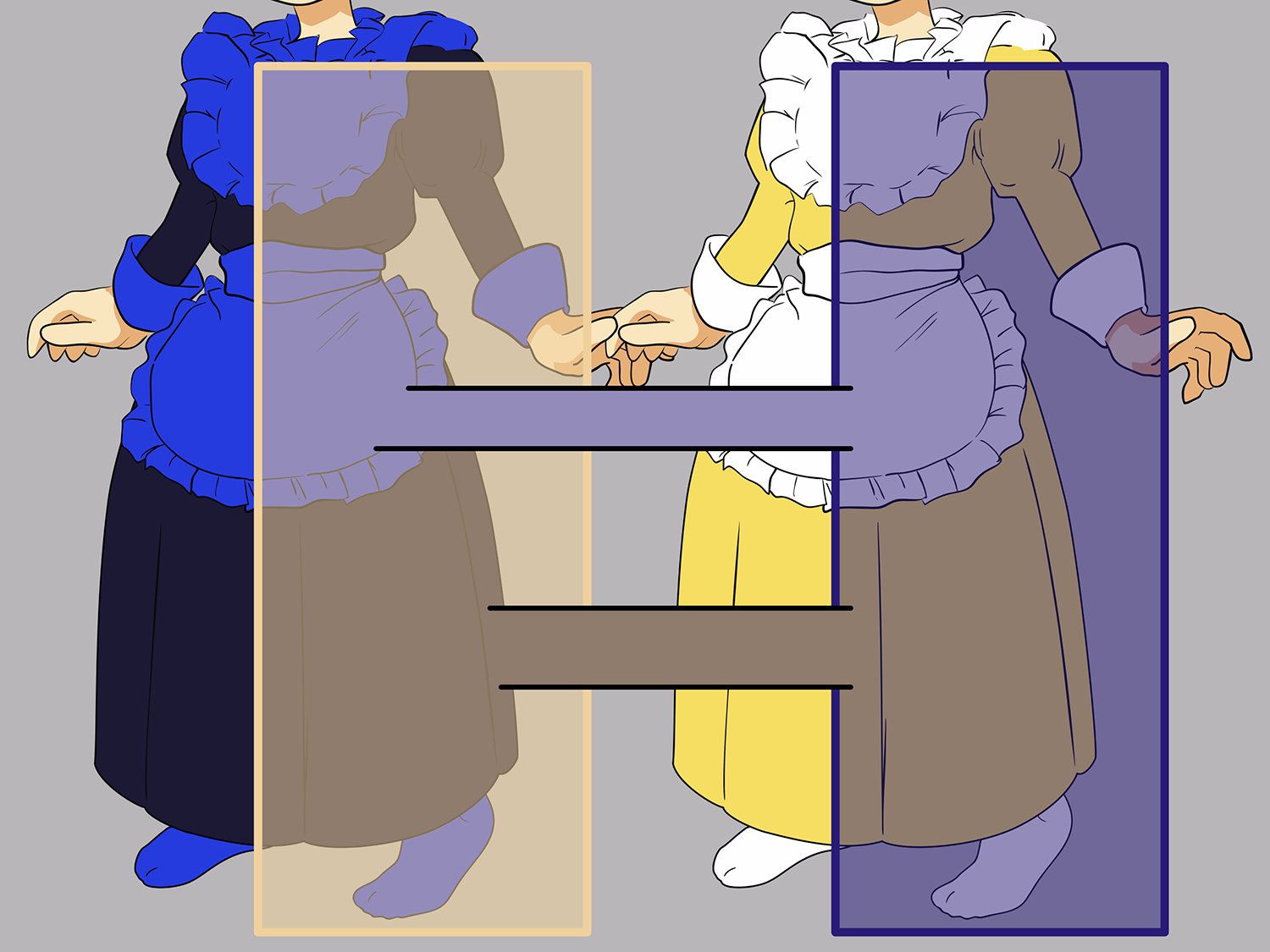
Illustration of the way different filters, corresponding to different assumptions about illumination, produce different interpretations of color in The Dress
Even between species, both a common biological toolkit and interlocking umwelten tend to reinforce a consensus reality. Our interests, hence our models, are all entangled, whether cooperatively or adversarially. Indeed, it can be hard to tell the difference. A rabbit that fails to effectively recognize and distinguish between fellow rabbits and wolves is not long for this world. Nor is a wolf who can’t recognize dinner. Over evolutionary time, through this apparently adversarial interaction, wolves and rabbits have cooperated to mutually shape each other’s highly capable bodies and sophisticated world models.
The science-fiction writer Philip K. Dick once wrote, “Reality is that which, when you stop believing in it, doesn’t go away.” 43 While an entity may ignore or variously interpret many of its input signals, failure to understand the relationship between those signals and its own future existence will result in future non-existence. At a minimum, then, facts are models that work well enough not to kill you.
Consensus is easier to achieve for X than for H. Two agents who (perhaps by virtue of both being human) have similar sensory apparatus, similar survival imperatives, share a common language, and are looking at the same dress, will in an overwhelming majority of cases agree on its color.
On the other hand, a hidden state H by definition is not directly accessible to an other. I can say that I’m hungry or tired or feel sad, but … you’ll just have to take my word for it. Or not. Under certain circumstances, it can be important for hidden states to remain hidden. Hence we become anxious when neuroscientists develop methods to “read out” hidden states in our brains, or social media companies seek to use algorithmic wizardry to infer our innermost desires. 44
Are Feelings Real?
The most rudimentary kinds of feelings are little more than physical signals: hunger, cold, heat, thirst. For any organism that seeks to stay alive—that is, for anything that is alive, as remaining so requires constant work—gauges and meters like these matter. Is it time to sweat, or to shiver? Pick the wrong answer, and your model might not be around to make any more janky predictions tomorrow.
For a bacterium, such gauges are chemical measurements, just like environmental variables; they’re simply assessing conditions on the inside of the cell membrane rather than the outside. That implies solving the same kind of computational problem as for an external measurement. Finding the correlation between a raw signal (like molecular docking and undocking events) and an estimated property (like concentration, or hunger) requires a learned, and likely adaptive, model. As organisms get more complex, both the signaling mechanism and the model required to infer a variable like “hunger” become more complex.
Consider pain. In his 2023 book The Experience Machine: How Our Minds Predict and Shape Reality, 45 philosopher Andy Clark—whose take on the larger subject of brains as predictors I agree with—describes a number of telling ways our pain models can malfunction. Amputees, for instance, can experience phantom limb pain. Similarly, many people live with chronic pain disorders, often beginning with an acute injury or illness but persisting long after the physical damage has healed.
On the other hand, many of us are familiar with receiving injuries, sometimes serious, that don’t hurt at first—the pain only comes later, if at all, and sometimes seems to depend on our higher-level awareness of the injury. To cite one gruesome example: in early 2005, a construction worker in Colorado experienced what he perceived as a bruising blow from a recoiling nail gun at a job site. Six days later, he visited the dentist, complaining of a mild toothache; he had been icing it and taking Advil. An x-ray revealed that he had fired a four inch nail through the roof of his mouth and into his brain. He recovered well following surgery to remove the nail, but this tabloid story doesn’t inspire me to take on more handyman stuff around the house. 46

X-ray of a four-inch nail embedded in the skull of twenty-three-year-old construction worker Patrick Lawler, removed at Littleton Adventist Hospital in Denver on January 14, 2005, six days after Lawler unknowingly shot himself with a nail gun.
There’s an opposite phenomenon too, in which intense pain accompanies a mistaken perception of injury. Consider another story about an unfortunate encounter between a construction worker and a nail, as reported in the British Medical Journal in 1995. 47 This worker jumped from some scaffolding onto a plank, failing to notice the seven-inch nail projecting up from it, which pierced clean through his boot, coming out the top. In agony, the construction worker was dosed with fentanyl and midazolam. But in the emergency room, when the doctors pulled out the nail and removed the boot, they found that the nail had passed harmlessly between his toes.
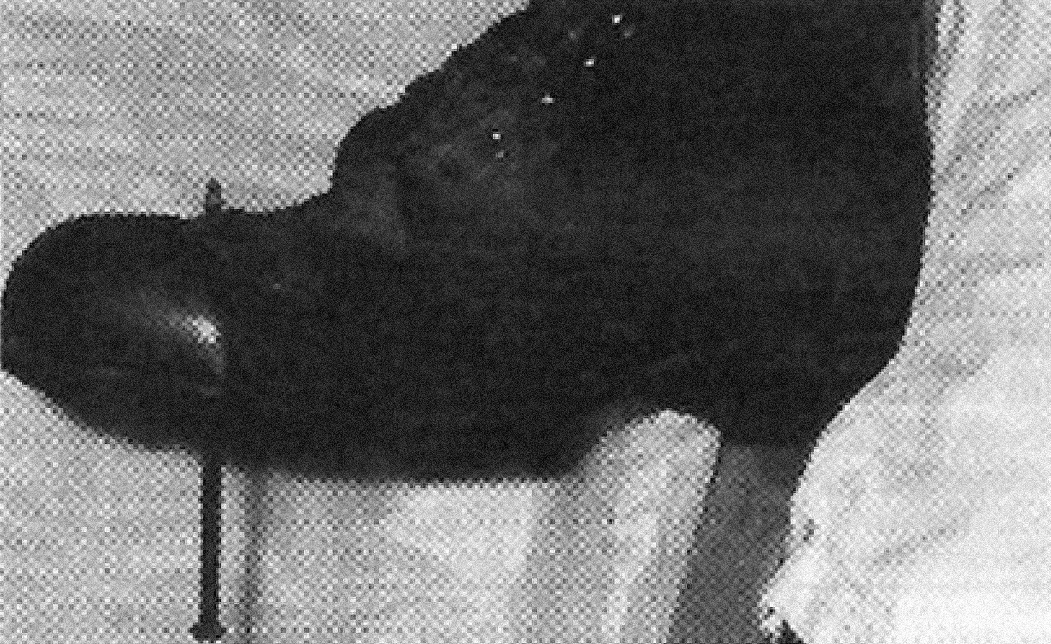
Boot of a twenty-nine-year-old construction worker pierced by a seven-inch nail, found at the hospital to have passed harmlessly between his toes, as reported in the British Medical Journal in 1995.
As Andy Clark puts it, “Such effects seem much less surprising once we accept that […] ‘raw’ sensory evidence is […] never experienced. […] [R]esponses of the ‘pain receptors’ (known as nociceptors) are not what we feel when we’re gripped by a sharp pain. Instead, those responses are simply one source of evidence […]. That’s why we can genuinely feel pain even when nociceptor activity is absent. We can also fail to feel pain even when intense nociceptor activity is present […]. What we feel […] reflects a process of unconscious inference […] about […] the events causing our sensory stimulations.” 48
Clark’s point is general: it’s not just about pain, but about the nature of reality, both external and internal, and how that “reality” is made. Beyond Hume’s “is/ought” distinction, Classical and Enlightenment dogma that reality can be cleanly separated from psychology is mistaken. The second construction worker was not faking pain, any more than the first construction worker was pretending not to be in much pain.
Neither Clark nor I would claim that reality doesn’t exist. Rather, we are using “reality” to describe a purposive model with a high degree of social consensus and good predictive power. We call the first construction worker’s belief that he was uninjured “false” because that belief would not have predicted the dramatic x-ray, or the urgent need for surgery. We call the second construction worker’s belief in his injury “false” because his belief would have predicted that, when the doctors removed his boot, they would find a bloody wound. When there was no such wound, everyone realized that their model needed updating; and, as a bonus, the man’s pain went away.
Unfortunately, it doesn’t always work so neatly. For people with chronic pain, knowing that nothing is “wrong” doesn’t bring relief—just as for people with arachnophobia, conscious knowledge that a pet tarantula is tame doesn’t make the dread of touching that giant hairy spider go away.
We’ve seen how even a virus needs an envelope, or it gives up the ability to exist outside its host cell and becomes a transposon.
Stock and Levit 2000 ↩.
Lazova et al. 2011 ↩.
Mathematical readers: to first order, if X is a sequence of discrete events, then to first order, P(X) will be a causal filter turning these discrete events into a continuous time-varying probability estimate. The elegant accuracy/latency tradeoffs bacteria perform (in effect, changing the filter shape) can be thought of as solving for the optimal linear prediction of X under changing statistical conditions.
The concept of a “thing in itself” (Ding an sich) comes from Immanuel Kant, who sought to distinguish an objective reality from our inevitably subjective or “phenomenal” experience of it; Kant 1998 ↩.
Wheeler 1992 ↩.
Although, to get ahead of our argument for a moment, how could that improbably chair-like configuration of atoms have come into existence in the first place, without any beings that model chairs?
Originally, Conway used a Go board. Go is an ancient strategy game, invented more than 2,500 years ago in China, involving two players alternately placing white and black stones at the unoccupied intersections on a 19×19 grid.
Loizeau 2021 ↩.
Bradbury 2012 ↩.
Technical caveat: to simulate quantum mechanics, a random number source would also be needed.
There is also the question of initial conditions, of which more anon.
This understanding or knowledge about the world of Life is consistent with, and even derivable from, the basic rules, just as statistical mechanics allows temperature and pressure to be derived from lower-level laws of elastically colliding particles in a box (which are themselves derivable from still more fundamental physics). It would be odd, though, to claim that gliders are “implied” or “inherent” in the rules of Life, for Life’s Turing completeness means that the complexity of the constructs possible in Life is unbounded; it includes anything and everything.
Niemiec 2010 ↩.
Hawking 2011 ↩.
By creating a numbering system that can enumerate all possible cellular automata, Stephen Wolfram and collaborators have started to explore the question of how “unusual” computation is in absolute terms. Rule number 110 has been proven to support computation—and many of the first hundred or so rules are so trivial that they create no meaningful dynamics at all. Observations like this, and the simplicity of Conway’s Life, suggest that a universe doesn’t need to be fine-tuned to support computation. See Wolfram 2002; Cook 2004 ↩, ↩.
Plants and fungi, life forms that lack muscles and so only move very slowly, should not be understood as passive. On the contrary, as the scientists who study them are increasingly appreciating, they compensate for immobility with the ability to take an extraordinary variety of chemical actions.
Technically, self-supervision involves turning an unsupervised task into a supervised one by somehow labeling the data with itself. The paradigmatic example is next-word prediction for training large language models.
More formally, the joint distribution P(X,H,O) includes the “marginal distributions” P(H) and P(X), which we would get by summing the joint distribution over (X,O) or (H,O), as well as conditional distributions.
Technical note: once evolution has “learned” how to endow organisms with “primary drives” like hunger, it can also learn to use these as internal oracles to power reinforcement learning and other, more sophisticated learning algorithms, for instance, as described in Keramati and Gutkin 2011 ↩. “Bootstrapping,” in chapter 4, will explain reinforcement learning and its relationship to the brain in more detail.
Dennett 2017b ↩.
More formally, it requires reducing the dimensionality of the distribution by factoring out invariant dimensions, per Tishby, Pereira, and Bialek 2000 ↩.
A 4K (3,840×2,160 pixel) video stream, compressed, is typically between eight and fourteen million bits per second.
This may not seem like much of a model, but it’ll do for modeling some simple things, like, with a negative w, the restoring force exerted by stretching a spring by distance x.
Although the distinction isn’t nearly as straightforward as it sounds, as discussed in “Élan Vital,” chapter 1.
Turing 1936 ↩.
I’ve written the programmer’s version with lowercase variable names because in mathematical notation, capital letters are generally used for “random variables” that can assume a whole distribution of values.
Hofstadter 2007 ↩.
Although this terminology is a bit confusing, machine learning practitioners refer to evaluation of their trained models as “inference.”
Turing 1948 ↩.
Setting aside other potential life in the universe, we’re on the cusp of this no longer being true on Earth, as AI models are now being used to design other AI models, per Duéñez-Guzmán et al. 2023 ↩.
This line of thinking suggests a potentially fertile research direction. Evolution-inspired approaches to learning today are mostly based on random mutation, per Salimans et al. 2017 ↩. But as we’ve seen, symbiogenesis is far more powerful as a source of productive novelty.
“In general” because group-level fitness benefits from individual sacrifice under certain circumstances, as with bees defending the hive. Also, in species like the octopus, where individuals breed over a single season and aren’t involved in raising the young, there’s no evolutionary pressure on survival after reproduction.
This is an alternative formulation of “Occam’s Razor,” which holds that, all things being equal, a simpler explanation is more likely to be true than a complicated one.
Wright 1972 ↩. Note to physicists: it’s possible to formulate physics in terms of “principles of least action” rather than equivalent dynamical laws. This would involve evaluating all possible trajectories of the boulder to find a minimum (or, occasionally, maximum) action solution, wherein the car gets squashed. One could argue that in the action formulation all effects precede their causes, per Tegmark 2018 ↩. In my view, though, by removing any notion of causal ordering, the least-action approach presupposes a timeless “block universe” with no role for concepts like “why” and “because.” We’ll return to this topic in “Will What You Will,” chapter 6.
Deacon 2012 ↩.
Per the broadening of terms suggested in “Élan Vital,” chapter 1, this definition of “purposive” or even “alive” includes technological systems with built-in decision-making powers, from thermostats to cruise missiles, as well as artificially evolved systems like bff.
Hume 1817 ↩.
Wallisch 2017 ↩.
Dick 1985 ↩.
A. Clark 2023 ↩.
A. Clark 2023 ↩.