Abiogenesis
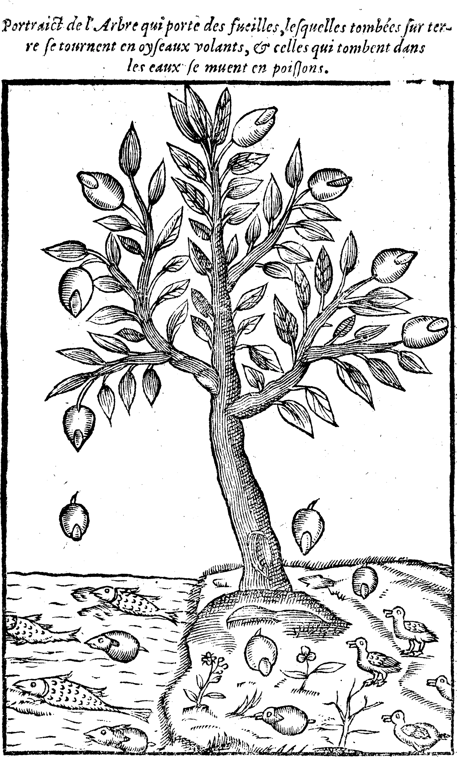
Spontaneous generation of birds and fish by a tree, depending on where its seeds land; Claude Duret, Histoire admirable des plantes et herbes esmerueillables et miraculeuses en nature, 1605
How did life on Earth begin? In the nineteenth century, this seemed like an unanswerable question. Researchers attempting to catch life in the act of “spontaneous generation” had come up empty-handed once they learned how to decontaminate their samples.
As William Thomson (1824–1907), the future Lord Kelvin, put it in an 1871 address before the British Association for the Advancement of Science, “Dead matter cannot become living without coming under the influence of matter previously alive. This seems to me as sure a teaching of science as the law of gravitation.” 1
Has life somehow always existed, then? Did it arrive on Earth from outer space, borne on an asteroid? Thomson thought so, and some still do. Not that this “panspermia” hypothesis really gets us anywhere. Where did the asteroid come from, and how did life arise there?
Despite his clear articulation of the principle of evolution, Charles Darwin (1809–1882) didn’t have a clue either. That’s why, in 1863, he wrote to his close friend Joseph Dalton Hooker that “it is mere rubbish, thinking, at present, of origin of life; one might as well think of origin of matter.” 2
Today, we have more of a clue, although the details may forever be lost to deep time.
Biologists and chemists working in the field of abiogenesis—the study of the moment when, billions of years ago, chemistry became life—have developed multiple plausible origin stories. In one, proto-organisms in an ancient “RNA world” were organized around RNA molecules, which could both replicate and fold into 3D structures that could act like primitive enzymes. 3 In an alternative “metabolism first” account, 4 life began without genes, likely in the rock chimneys of “black smokers” on the ocean floor; RNA and DNA came later. It may eventually be possible to rule one or the other theory out … or it may not.
We’ll return to RNA and replication, but let’s begin by unpacking the metabolism-first version in some detail, as it sheds light on the problem that confounded Darwin and his successors: how evolution can get off the ground without genetic heritability. As we’ll see, abiogenesis becomes less puzzling when we develop a more general understanding of evolution—one that can extend back to the time before life.
Lava lake, Kīlauea, Hawai‘i
Let’s cast our minds back to our planet’s origins. The Hadean Eon began 4.6 billion years ago, when the Earth first condensed out of the accretion disc of rocky material orbiting our newborn star, the Sun. Our planet’s mantle, runnier than it is today and laden with hot, short-lived radioactive elements, roiled queasily, outgassing carbon dioxide and water vapor. The surface was a volcanic hellscape, glowing with lakes of superheated lava and pocked with sulfurous vents belching smoke.
It took hundreds of millions of years for surface conditions to settle down. According to the International Astronomical Union, an object orbiting a star can only be considered a planet if it has enough mass to either absorb or, in sweeping by, to eject other occupants from its orbit. But in the chaos of the early Solar system, this took a long time. While Earth was clearing its orbit of debris, it was continually bombarded by comets and asteroids, including giant impactors more than sixty miles across. A single such impact would have heated the already stifling atmosphere to a thousand degrees Fahrenheit.
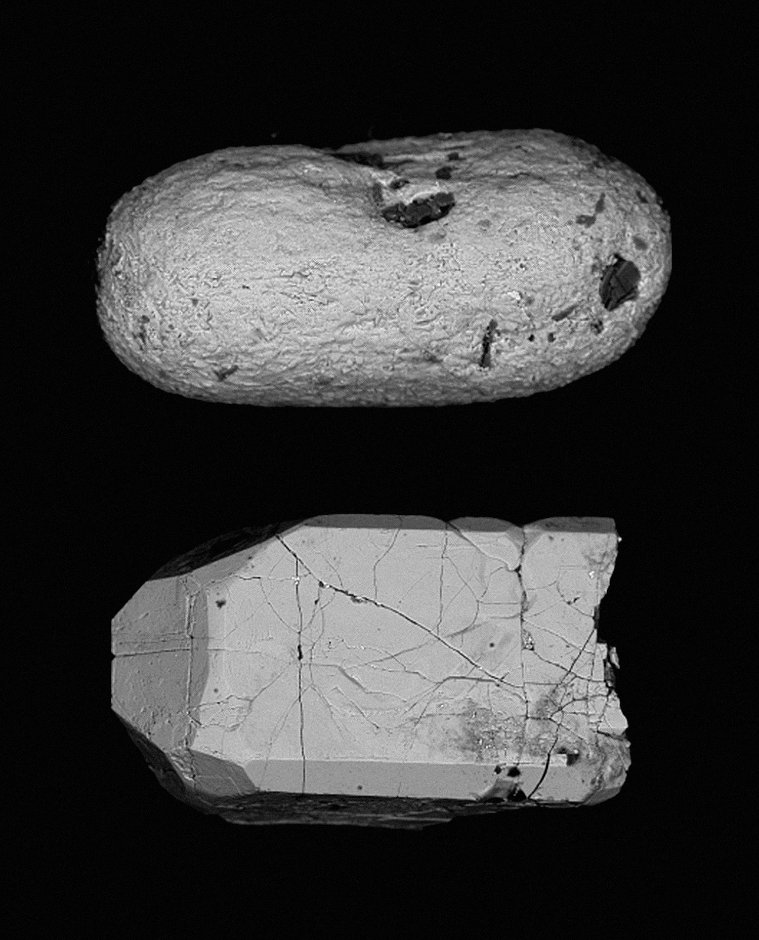
Backscatter electron micrograph of 4.4-billion-year-old detrital zircons from the Hadean metasediments of the Jack Hills, Narryer Gneiss Terrane, Western Australia
One of those collisions appears to have been with another newly formed planet, an event that came close to destroying the Earth altogether. According to this theory, enough broken, liquefied, and vaporized rock splashed into orbit to coalesce into the Moon.
Unsurprisingly, very little geological material survives from the Hadean—mainly zircon crystals embedded within metamorphic sandstone in the Jack Hills of Western Australia.
It’s difficult to imagine anything like life forming or surviving under such harsh conditions. Maybe, somehow, it did. We know for sure that by later in the Hadean or the early Archean—3.6 billion years ago, at the latest—the surface had cooled enough for a liquid ocean to condense and for the chemistry of life to begin brewing.
Today, those early conditions are most closely reproduced by black smokers. These form around hydrothermal vents on the mid-ocean ridges where tectonic plates are pulling apart and new crust is forming. In such places, seawater seeping down into the rock comes into contact with hot magma. Superheated water then boils back up, carrying hydrogen, carbon dioxide, and sulfur compounds, which precipitate out to build smoking undersea chimneys. Probes sent thousands of feet down to explore these otherworldly environments find them teeming with weird life forms of all kinds, attracted by warmth, nutrients, and each other. Some of the inhabitants may go a long, long way back.
The “Candelabra” black smoker in the Logatchev hydrothermal field on the Mid-Atlantic Ridge, at a depth of 10,800 feet
Like lava rock, the chimneys are porous, and the pores are ideal little chambers for contained chemical reactions to take place—potentially powered by a handy energy source, since the hydrogen gas creates proton gradients across the thin walls between pores, making them act like batteries. 5 Given energy, iron sulfide minerals in the rock acting as catalysts, and carbon dioxide bubbling through, self-perpetuating loops of chemical reactions can sputter to life, like a motor turning over.
Perhaps this was life’s original motor: a primitive but quasi-stable metabolism, as yet without genes, enzymes, or even a clearly defined boundary between inside and outside. Such upgrades might have followed before long, though, for that chemical synthesis motor closely resembles the “reverse Krebs cycle,” now widely believed to have powered the earliest cells.
The ordinary or “forward” Krebs cycle was discovered in 1937 by groundbreaking biochemist Hans Krebs (1900–1981). More like a gas-powered generator than a motor, the Krebs cycle is at the heart of how all aerobic organisms on Earth “burn” organic fuels to release energy, a process known as “respiration.” 6 Inputs to this cycle of chemical reactions include complex organic molecules (which we eat) and oxygen (which we inhale); the “exhaust” contains carbon dioxide and water (which we exhale). The energy produced maintains proton gradients across folded-up membranes inside our mitochondria, and the flow of these protons goes on to power every other cellular function.
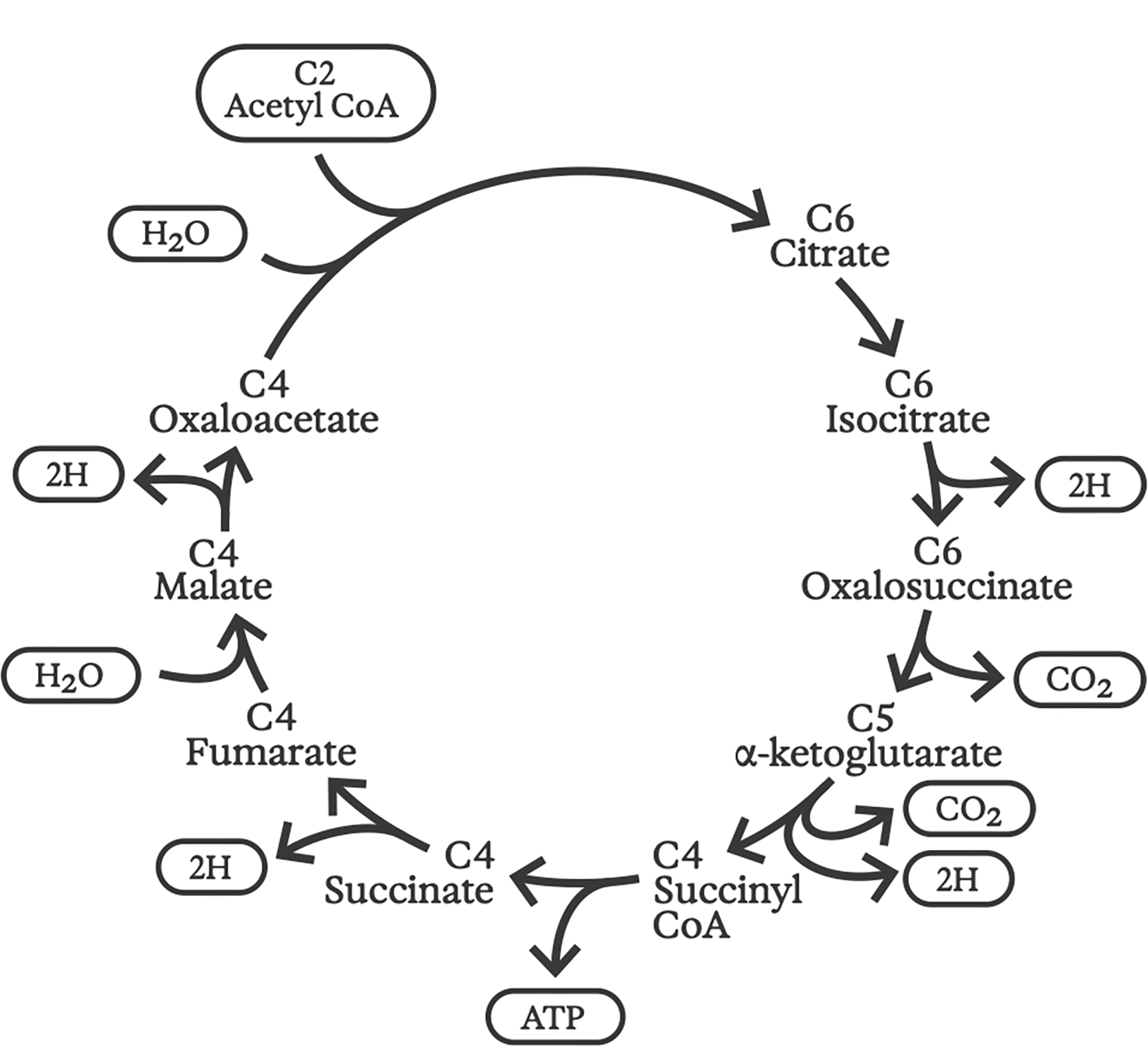
Krebs cycle
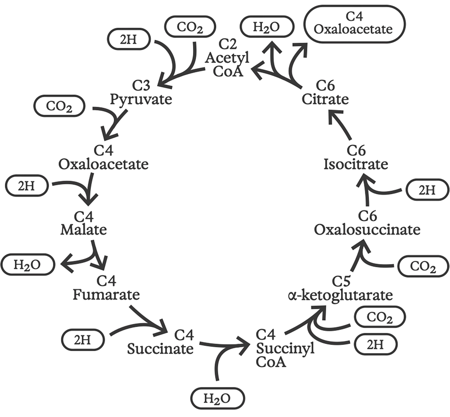
Reverse Krebs cycle
The idea of a “reverse Krebs cycle” was first proposed by a trio of researchers at UC Berkeley in 1966. 7 It remained controversial for decades, but is now known to power carbon fixation in ancient anaerobic sulfur bacteria—some of which still make their homes in deep-sea hydrothermal vents. 8 As its name implies, the reverse Krebs cycle consists of roughly the same chemical reactions as the forward cycle, but running in the opposite direction. Starting with water and carbon dioxide, proton gradients drive the synthesis of all of the basic building blocks needed for cellular structure and function, including sugars, amino acids for proteins, fatty acids and isoprenes for cell membranes, and nucleotides for building RNA and DNA. 9

X-ray of Russian matryoshka dolls
All life came from the sea, and the interior of every cell in every living organism reproduces that salty, watery environment—a tiny “ocean inside.” This much is common knowledge. But our mitochondria, the “power plants” within our cells where respiration takes place, may in fact be recapitulating the much more specific deep-sea chemistry of a black smoker. In an almost literal sense, our bodies are like Russian matryoshka dolls, membranes within membranes, and each nested environment recreates an earlier stage in the evolution of life on Earth.
The deeper inside ourselves we look, the farther we can see into the past. A beautiful, shivery thought.
Symbiogenesis
Whether RNA or metabolism came first, even the simplest bacteria surviving today are a product of many subsequent evolutionary steps. Yet unlike the everyday, incremental mutation and selection Darwin imagined, the most important of these steps may have been large and sudden. These “major evolutionary transitions” involve simpler, less complex replicating entities becoming interdependent to form a larger, more complex, more capable replicator. 10
Transmission electron microscopy showing mitochondria in cells
As maverick biologist Lynn Margulis (1938–2011) discovered in the 1960s, eukaryotic cells, like those that make up our bodies, are the result of such an event. Roughly two billion years ago, the bacteria that became our mitochondria were engulfed by another single-celled life form 11 much like today’s archaea—tiny, equally ancient microorganisms that continue to inhabit extreme environments, like hot springs and deep-sea vents. This is “symbiogenesis,” the creation or genesis of a new kind of entity out of a novel “symbiosis,” or mutually beneficial relationship, among pre-existing entities.
At moments like these, the tree of life doesn’t just branch; it also entangles with itself, its branches merging to produce radically new forms. Margulis was an early champion of the idea that these events drive evolution’s leaps forward.
It’s likely that bacteria are themselves the product of such symbiotic events—for instance, between RNA and metabolism. 12 RNA could replicate without help from proteins, and the metabolic motor could proliferate without help from genes, but when these systems cooperate, they do better. The looping chemical-reaction networks in those black smokers can be understood as such an alliance in their own right, a set of reactions which, by virtue of catalyzing each other, can form a more robust, self-sustaining whole.
So in a sense, Darwin may have been right to say that “it is mere rubbish” to think about the origin of life, for life may have had no single origin, but rather, have woven itself together from many separate strands, the oldest of which look like ordinary chemistry. Intelligent design is not required for that weaving to take place; only the incontrovertible logic that sometimes an alliance creates something enduring, and that whatever is enduring … endures.
Often, enduring means both creating and occupying entirely new niches. Hence eukaryotes did not replace bacteria; indeed, they ultimately created many new niches for them. Likewise, the symbiotic emergence of multicellular life—another major evolutionary transition—did not supplant single-celled life. Like an ancient parchment overwritten by generations of scribes, our planet is a palimpsest, its many-layered past still discernible in the present. Even the black smokers, throwbacks to a Hadean sea billions of years ago, are still bubbling away in the depths. The self-catalyzing chemistry of proto-life may still be brewing down there, slowly, on the ocean floor.
The idea that evolution is driven by symbiotic mergers, the earliest of which preceded biology as we know it, has far-reaching implications. One is that the boundary between life and non-life is not well defined; symbiogenesis can involve any process that, one way or another, is self-perpetuating. Evolutionary dynamics are thus more like a physical law than a biological principle. Everything is subject to evolution, whether we consider it to be “alive” or not.
The symbiogenetic view also renders the idea of distinct species, classified according to a Linnaean taxonomy, somewhat ill-defined—or at best, of limited applicability. Such taxonomies assume that only branching takes place, not merging. Bacteria, which promiscuously transfer genes even between “species,” already challenge this idea. 13 Taxonomies break down entirely when we try to apply them to even more fluid situations, like the possible proto-life in black smokers, or microbiomes, or the more complex symbioses we’ll explore later.
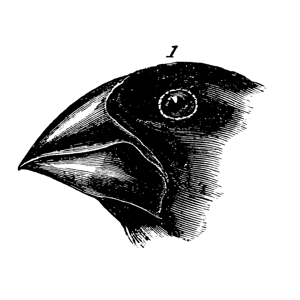
Galapagos finches, from Darwin, Voyage of the Beagle, 1845
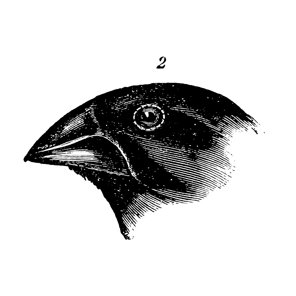
Galapagos finches, from Darwin, Voyage of the Beagle, 1845
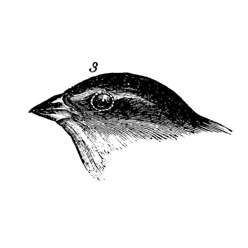
Galapagos finches, from Darwin, Voyage of the Beagle, 1845
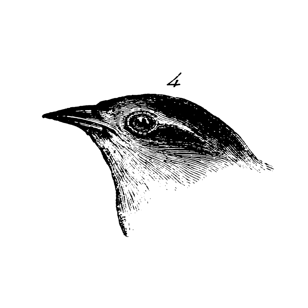
Galapagos finches, from Darwin, Voyage of the Beagle, 1845
Perhaps most importantly, symbiogenesis explains evolution’s arrow of time, as classical Darwinian theory alone cannot. When life branches, specializing to adapt to a niche—like Darwin’s finches with their differently shaped beaks, each optimized for a specific food source—those branches are in general no more complex than their ancestral form. This has led some classical evolutionary theorists to argue that the increasing complexity of life on Earth is an anthropocentric illusion, nothing more than the result of a random meander through genetic possibilities. 14 Relatedly, one sometimes hears the claim that since all extant species are of equal age—as it seems they must be, since all share a common single-celled ancestor some four billion years ago—no species is more “evolved” than any other.
On its face, that seems reasonable. But as we’ve seen, classical Darwinian theory struggles to explain why life seems to become increasingly complex, or, indeed, how life could arise in the first place. In themselves, random changes or mutations can only fine-tune, diversify, and optimize, allowing the expression of one or another variation already latent in the genetic space. (The space of possible finch beaks, for instance.)
When one prokaryote ends up living inside another, though, or multiple cells band together to make a multicellular life form, the resulting composite organism is clearly more complex than its parts. Something genuinely new has arisen. The branching and fine-tuning of classical evolution can now start to operate on a whole different level, over a new space of combinatorial possibilities.
Classical evolution isn’t wrong; it just misses half of the story—the more rapid, more creative half. One could say that evolution’s other half is revolution, and that revolutions occur through symbiosis.
Suggestively, the same is true of technology. In Paleolithic times, a hafted spear was not just a specialized stone point, but something new that arose by combining at least three parts: a stone point, a shaft, and something like sinew to bind them. This, too, opened up a new combinatorial design space. Or, in more recent times, the silicon chip was not just an evolved transistor; it was something new that could be made by putting multiple transistors together on the same die. One doesn’t arrive at chip design merely by playing with the design parameters of an individual transistor.
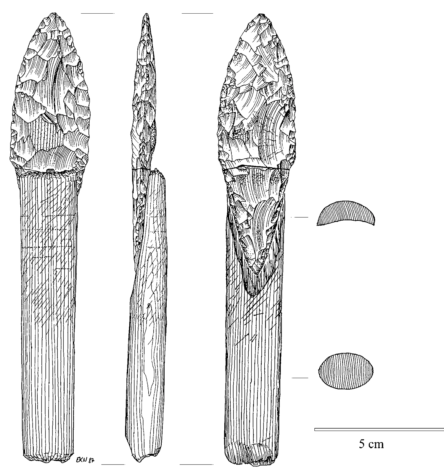
Hafted spear point from the mid-Holocene Arctic Small Tool site of Qeqertasussuk, West Greenland. Drawn by Eva Koch, reproduced with permission of Bjarne Grønnow.
That’s why evolution progresses from simpler to more complex forms. It’s also why the simpler forms often remain in play even after a successful symbiogenetic event. Standalone stone points, like knives and hand axes, were still being made after the invention of the hafted spear; and, of course, spearheads themselves still count as stone points. 15 Moreover, no matter how recently any particular stone point was made, we can meaningfully talk about stone points being “older” as a category than spears. Spears had to arise later, because their existence depended on the pre-existence of stone points.
It’s equally meaningful to talk about ancient life forms, like bacteria and archaea, co-existing alongside recent and far more complex ones, like humans—while recognizing that humans are, in a sense, complex colonies of bacteria and archaea that have undergone a cascade of symbiotic mergers.
Reproductive Functions
While most biochemists have focused on understanding the particular history and workings of life on Earth, a more general understanding of life has come from an unexpected quarter: computer science. The theoretical foundations of this surprising connection date back to those two founding figures of the field, Alan Turing and John von Neumann.
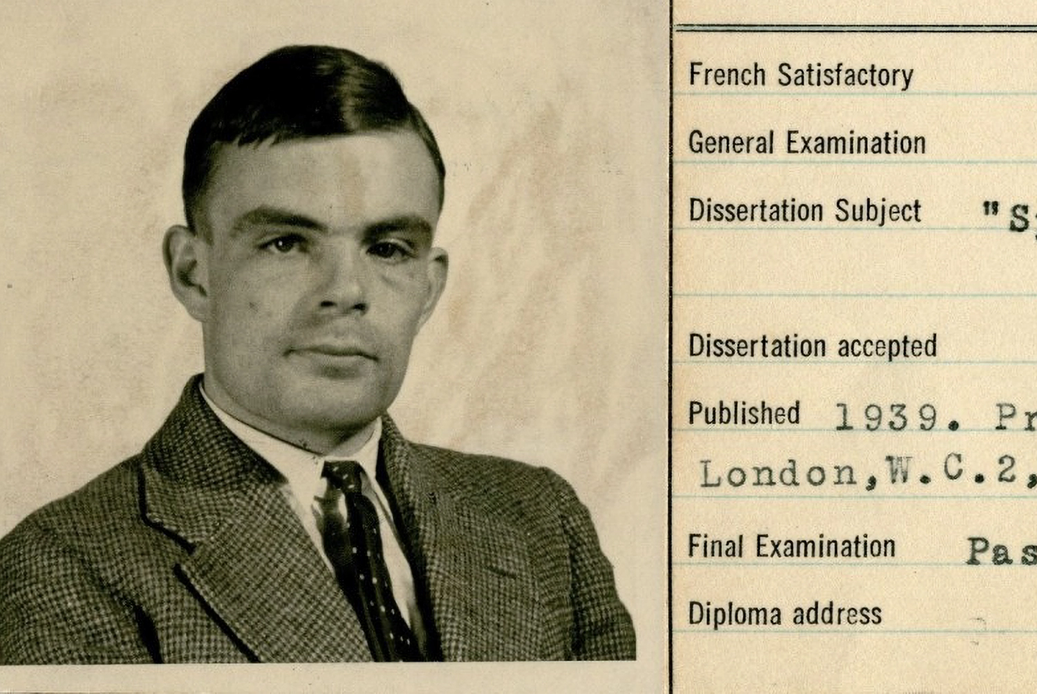
Alan Turing at Princeton University
I’ve already mentioned Turing’s 1950 paper introducing the Imitation Game or Turing Test, but his first great contribution came fifteen years earlier. After earning an undergraduate degree in mathematics at Cambridge in 1935, Turing focused on one of the fundamental outstanding problems of the day: the Entscheidungsproblem (German for “decision problem”), which asked whether there exists an algorithm for determining the validity of an arbitrary mathematical statement.
The answer turned out to be “no,” but the way Turing went about proving it ended up being far more important than the result itself—which was lucky, since American mathematician Alonzo Church had just scooped Turing, publishing his own proof a few months earlier using a different approach. 16 After corresponding with him about the Entscheidungsproblem, Turing would end up moving to Princeton to become Church’s doctoral student.
Proving mathematical statements about mathematical statements requires defining a general notation for such statements, and a procedure for evaluating them. Church did so using mathematical symbols, especially the lowercase Greek letter λ (lambda), thus inventing a self-referential “lambda calculus.”
Von Neumann illustrates a Turing machine at the start of his third 1945 lecture on high-speed computing machines
Turing took a less conventional route. His procedure involved an imaginary gadget we now call the “Turing Machine.” The Turing Machine consists of a read/write head, which can move left or right along an infinite tape, reading and writing symbols on the tape according to a set of rules specified by a built-in table.
First, Turing showed that such a machine could do any calculation or computation that can be done by hand, given an appropriate table of rules, enough time, and enough tape. He suggested a notation for writing down the table of rules, which he referred to as a machine’s “Standard Description” or “S. D.” Today, we’d call it a “program.”
Then, the really clever part: if the program itself is written on the tape, there exist particular tables of rules that will read the program and perform whatever computation it specifies. Today, these are called “Universal Turing Machines.” In Turing’s more precise language, “It is possible to invent a single machine which can be used to compute any computable sequence. If this machine U is supplied with a tape on the beginning of which is written the S. D. of some computing machine M, then U will compute the same sequence as M.”
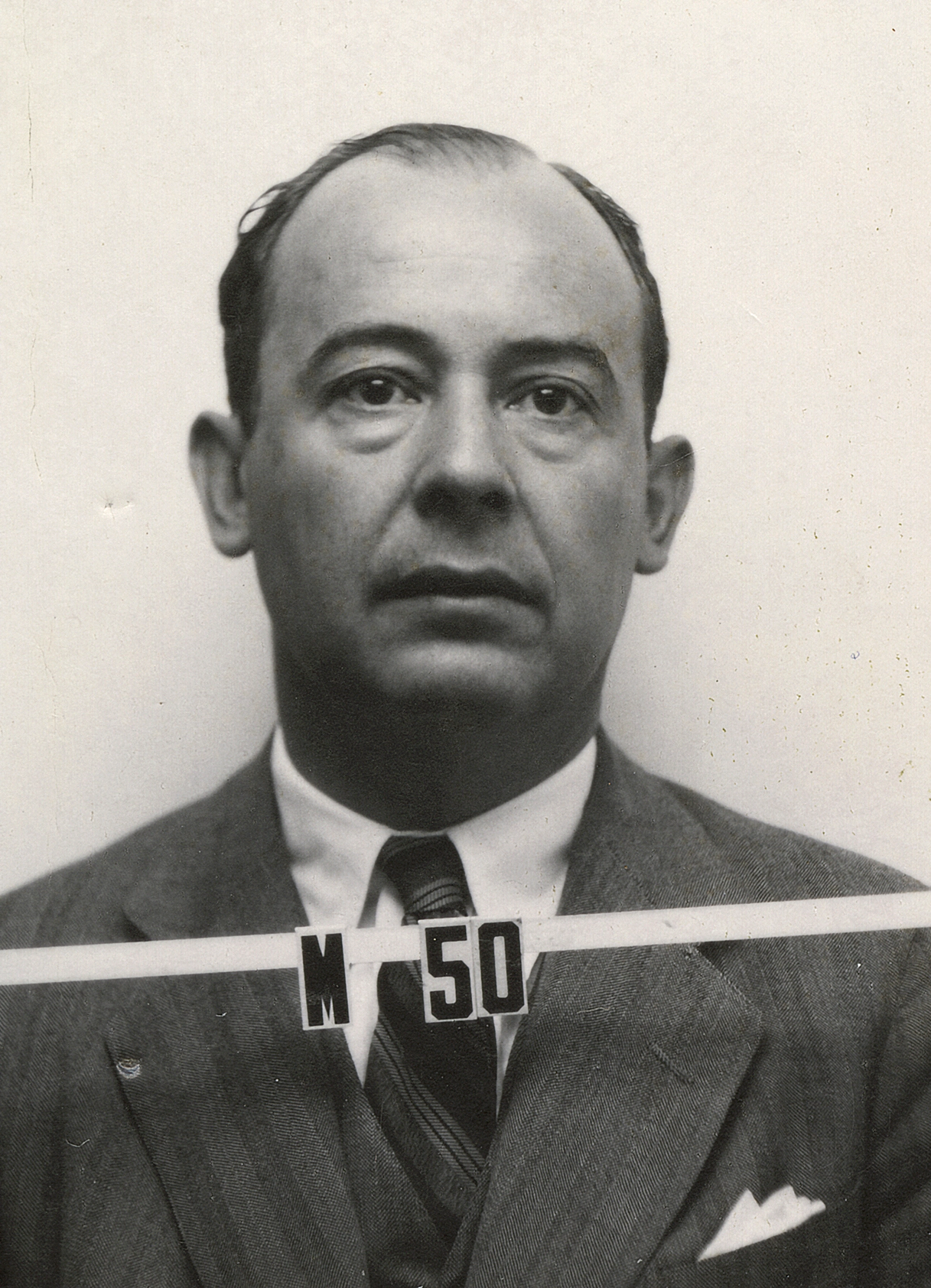
John von Neumann’s Los Alamos ID badge photo, 1940s
Some programs run for a time, then finish. Others run forever. Since a Universal Turing Machine allows programs themselves to be expressed as values on the tape, a program can take another program as input. One can imagine such a “meta-program” outputting a single bit of information that denotes whether the inputted program will eventually finish, or will keep running forever. Turing called this the “halting problem.” In his 1936 paper, he proved that a program that solves the halting problem for all possible input programs—and that is itself guaranteed to halt—is a logical impossibility. This was the result that answered the Entscheidungsproblem in the negative.
More consequentially, though, the Universal Turing Machine defined a generic procedure for computation. Turing was soon able to prove that any function that could be computed by his imaginary machine could also be expressed in Church’s lambda calculus, and vice versa 17 —a cornerstone of the idea now known as the Church-Turing thesis: that computability is a universal concept, regardless of how it’s done.
In the early 1940s, John von Neumann, a Hungarian American polymath who had already made major contributions to physics and mathematics, turned his attention to computing. He became a key figure in the design of the ENIAC and EDVAC—among the world’s first real-life Universal Turing Machines, now known simply as “computers.” 18
Turning an imaginary mathematical machine into a working physical one required many further conceptual leaps, in addition to a lot of hard nuts-and-bolts engineering. For instance, over the years, much creativity has gone into figuring out how simple the “Standard Description” of a Universal Turing Machine can get. Only a few instructions are needed. Esoteric language nerds have even figured out how to compute with a single instruction (a so-called OISC or “one-instruction set computer”).
There are irreducible requirements, though: the instruction, or instructions, must change the environment in some way that subsequent instructions are able to “see,” and there must be “conditional branching,” meaning that depending on the state of the environment, either one thing or another will happen. In most programming languages, this is expressed using “if/then” statements. When there’s only a single instruction, it must serve both purposes, as with the SUBLEQ language, whose only instruction is “subtract and branch if the result is less than or equal to zero.”
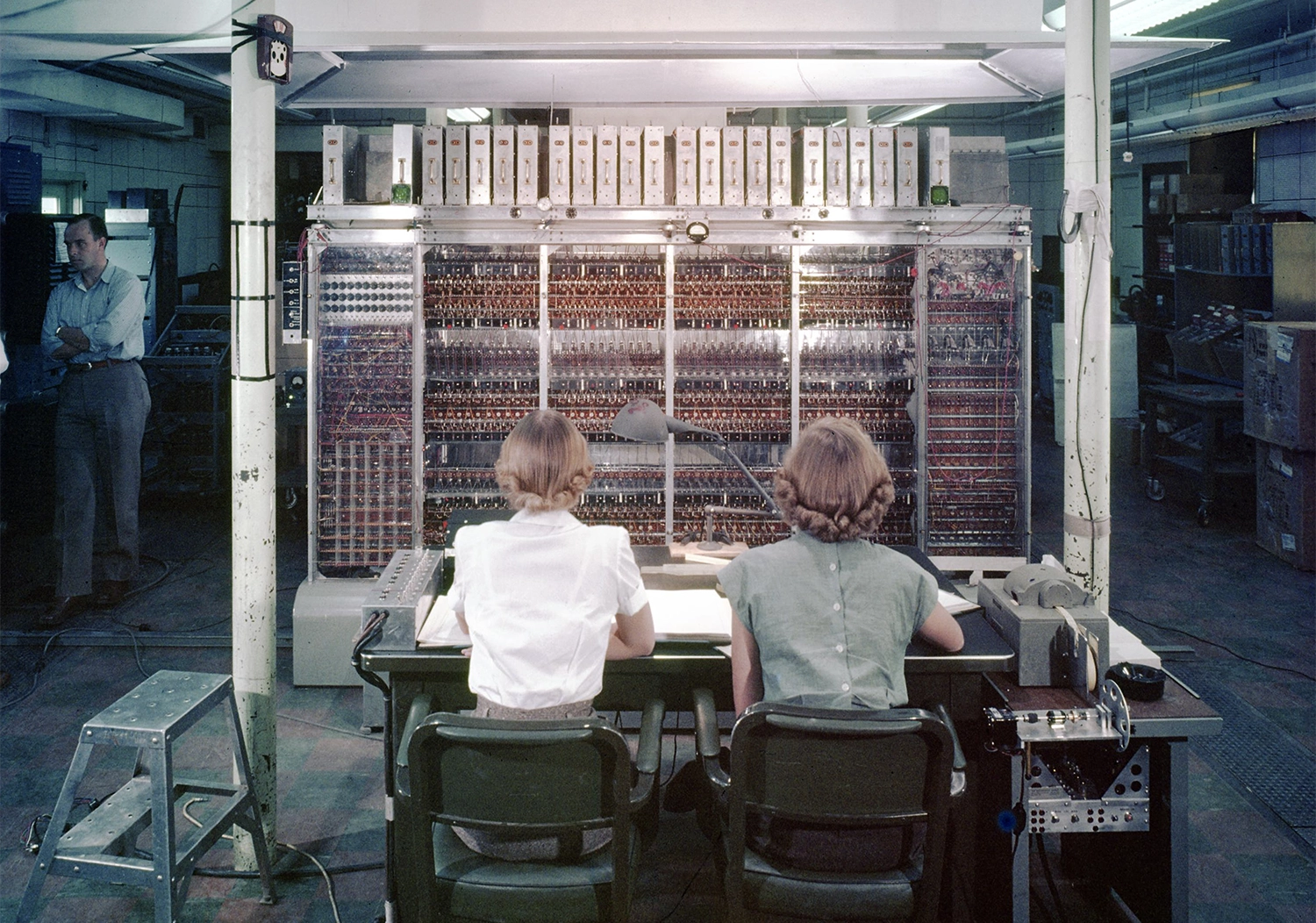
Programmers in front of the MANIAC computer, Los Alamos National Lab, 1952
Both Turing and von Neumann were keenly aware of the parallels between computers and brains. Von Neumann’s report on the EDVAC explicitly described the machine’s basic building blocks, its “logic gates,” as electronic neurons. 19 Whether or not that analogy held (as we’ll see, it did not; neurons are more complex than logic gates), his key insight was that both brains and computers are defined not by their mechanisms, but by what they do—their function, in both the colloquial and mathematical sense.
In real life, though, the brain is not an abstract machine, but part of the body, and the body is part of the physical world. How can one speak in purely computational terms about the function of a living organism, when it must physically grow and reproduce?
Although working independently, toward the end of their lives, Turing and von Neumann both became captivated by the connection between biology and computation. 20 Turing did pioneering work in “morphogenesis,” working out how cells could use chemical signals, which he dubbed “morphogens,” to form complex self-organizing patterns—the key to multicellularity. 21 Although computers were still too primitive to carry out any detailed simulations of such systems, he showed mathematically how so-called “reaction-diffusion” equations could generate spots, like those on leopards and cows, or govern the growth of tentacles, like those of the freshwater polyp, Hydra. 22
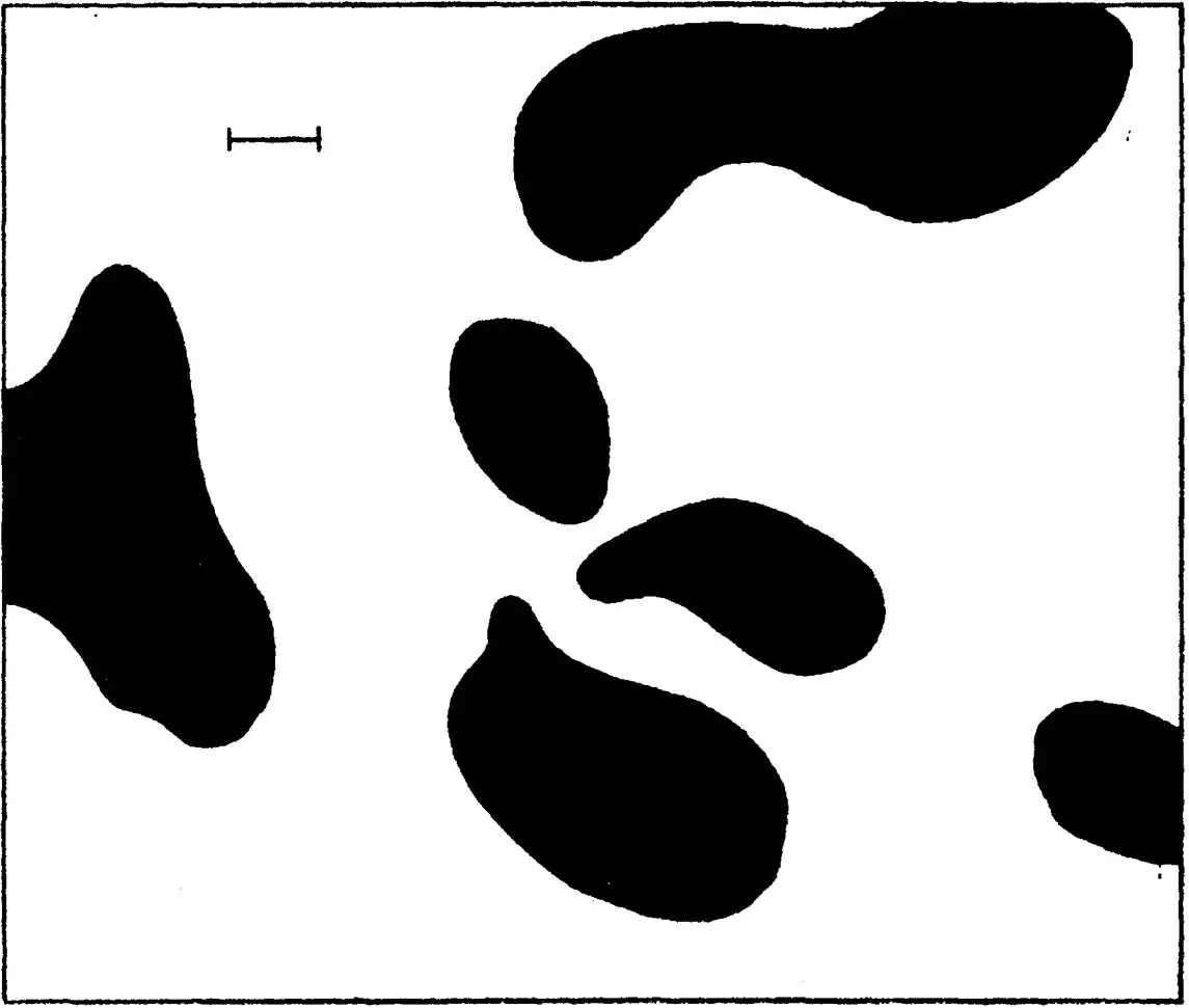
Reaction–diffusion pattern from Turing, “The Chemical Basis of Morphogenesis,” 1952
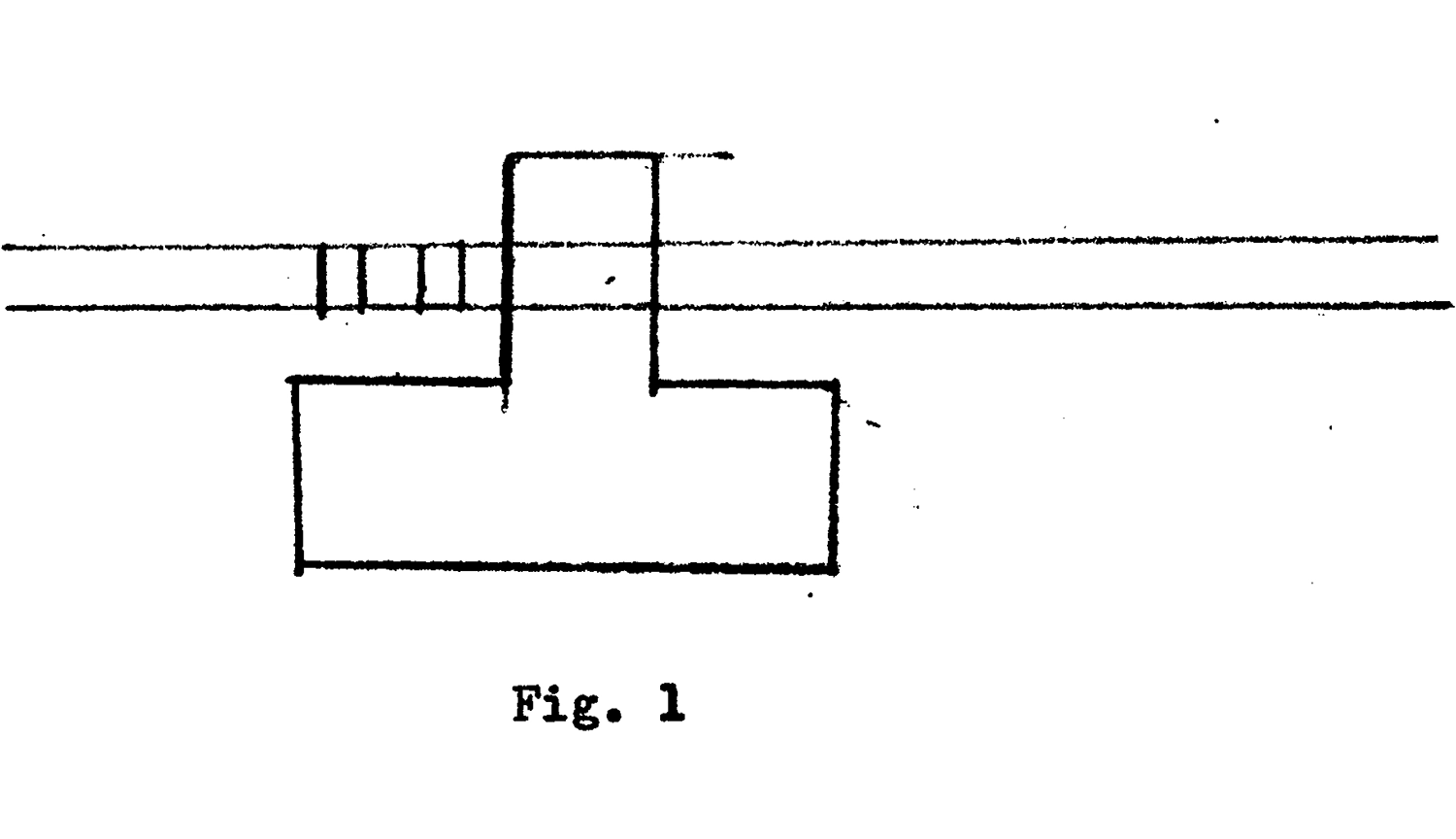
Around the same time, in a 1951 paper, 23 von Neumann imagined a machine made of standardized parts, like Lego bricks, paddling around on a reservoir where those parts could be found bobbing on the water. The machine’s job was to gather all of the needed parts and construct another machine like itself. Of course, that’s exactly what a bacterium does to reproduce; in fact it’s what every cell must do to divide, and what every mother must do to give birth.
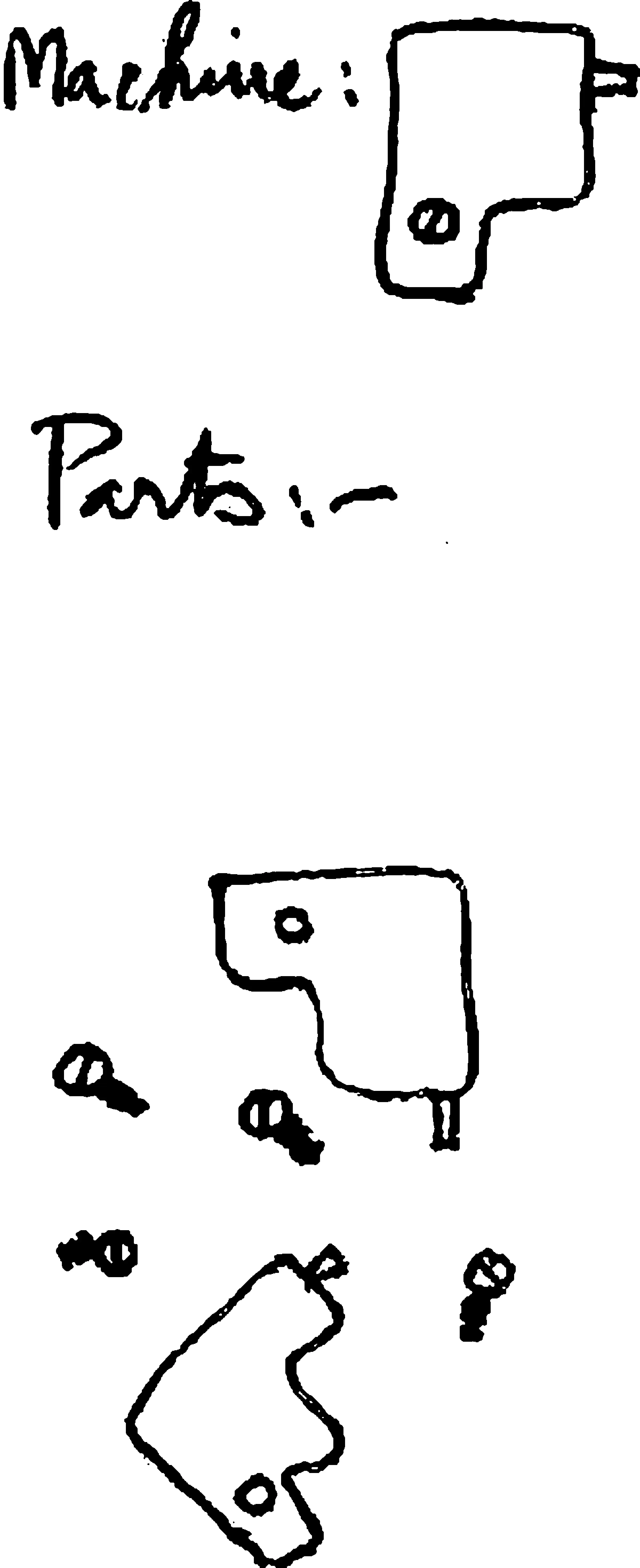
Note on self-reproducing machinery from the notebook of cybernetics pioneer W. Ross Ashby, December 22, 1954
It’s possible for a trivially simple structure, like a seed crystal, to “reproduce” merely by acting as a template for more of the same stuff to crystallize around it. But a complex machine—one with any internal parts, for example—can’t serve as its own template. And if you are a complex machine, then, on the face of it, manufacturing something just as complex as you yourself are has a whiff of paradox, like lifting yourself up by your own bootstraps. However, von Neumann showed that it is not only possible, but straightforward, using a generalization of the Universal Turing Machine.
He envisioned a “machine A” that would read a tape containing sequential assembly instructions based on a limited catalog of parts, and carry them out, step by step. Then a “machine B” would copy the tape—assuming the tape itself was also made of available parts. If instructions for building machines A and B are themselves encoded on the tape, then voilà—you would have a replicator. 24
Instructions for building any additional non-reproductive machinery could also be encoded on the tape, so it would even be possible for a replicator to build something more complex than itself. 25 A seed, or a fertilized egg, illustrates the point. Even more fundamentally, encoding the instructions to build oneself in a form that is itself replicated (the tape) is the key to open-ended evolvability, meaning the ability for evolution to select for an arbitrary design change, and for that change to be inherited by the next generation.
Remarkably, von Neumann described these requirements for an evolvable, self-replicating machine before the discovery of DNA’s structure and function. 26 Nonetheless, he got it exactly right. For life on Earth, DNA is the tape; DNA polymerase, which copies DNA, is “machine B”; and ribosomes, which build proteins by following the sequentially encoded instructions on DNA, are “machine A.” Ribosomes and DNA polymerase are made of proteins whose sequences are, in turn, encoded in our DNA and manufactured by ribosomes. That is how life lifts itself up by its own bootstraps.
Life as Computation
Although this is seldom fully appreciated, von Neumann’s insight established a profound link between life and computation. Remember, machines A and B are Turing Machines. They must execute instructions that affect their environment, and those instructions must run in a loop, starting at the beginning and finishing at the end. That requires branching, such as “if the next instruction is the codon CGA then add an arginine to the protein under construction,” and “if the next instruction is UAG then STOP.” It’s not a metaphor to call DNA a “program”—that is literally the case.
Of course, there are meaningful differences between biological computing and the kind of digital computing done by the ENIAC or your smartphone. DNA is subtle and multilayered, including phenomena like epigenetics and gene proximity effects. Cellular DNA is nowhere near the whole story, either. Our bodies contain (and continually swap) countless bacteria and viruses, each running their own code.
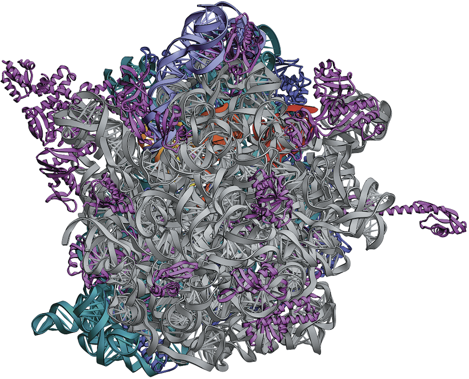
Structure of the 70S ribosome
Biological computing is “massively parallel,” decentralized, and noisy. Your cells have somewhere in the neighborhood of three hundred quintillion ribosomes, all working at the same time. Each of these exquisitely complex floating protein factories is, in effect, a tiny computer—albeit a stochastic one, meaning not entirely predictable. The movements of hinged components, the capture and release of smaller molecules, and the manipulation of chemical bonds are all individually random, reversible, and inexact, driven this way and that by constant thermal buffeting. Only a statistical asymmetry favors one direction over another, with clever origami moves tending to “lock in” certain steps such that a next step becomes likely to happen. This differs greatly from the operation of logic gates in a computer, which are irreversible, 27 and designed to be ninety-nine point many-nines percent reliable and reproducible.
Biological computing is computing, nonetheless. And its use of randomness is a feature, not a bug. In fact, many classic algorithms in computer science also require randomness (albeit for different reasons), which may explain why Turing insisted that the Ferranti Mark I, an early computer he helped to design in 1951, include a random number instruction. 28 Randomness is thus a small but important conceptual extension to the original Turing Machine, though any computer can simulate it by calculating deterministic but random-looking or “pseudorandom” numbers.
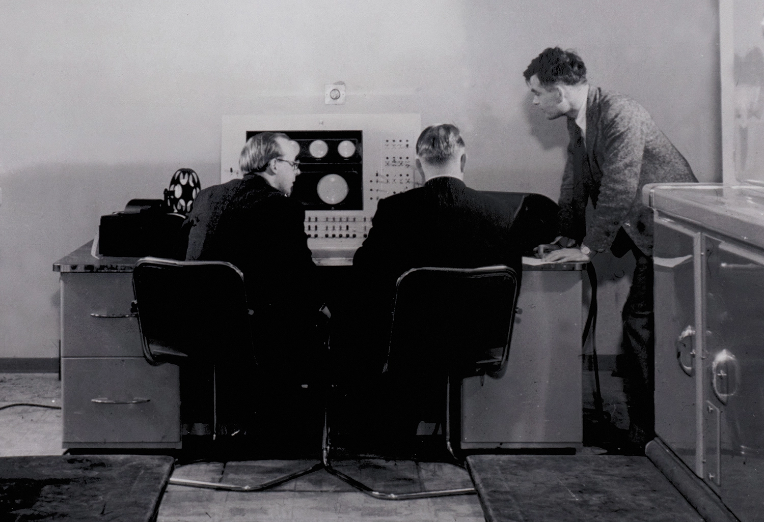
Turing (right) at the console of the Ferranti Mark II computer
Parallelism, too, is increasingly fundamental to computing today. Modern AI, for instance, depends on both massive parallelism and randomness—as in the parallelized “stochastic gradient descent” (SGD) algorithm, used for training most of today’s neural nets, the “temperature” setting used in chatbots to introduce a degree of randomness into their output, and the parallelism of Graphics Processing Units (GPUs), which power most AI in data centers.
Traditional digital computing, which relies on the centralized, sequential execution of instructions, was a product of technological constraints. The first computers needed to carry out long calculations using as few parts as possible. Originally, those parts were flaky, expensive vacuum tubes, which had a tendency to burn out and needed frequent replacement by hand. The natural design, then, was a minimal “Central Processing Unit” (CPU) operating on sequences of bits ferried back and forth from an external memory. This has come to be known as the “von Neumann architecture.”
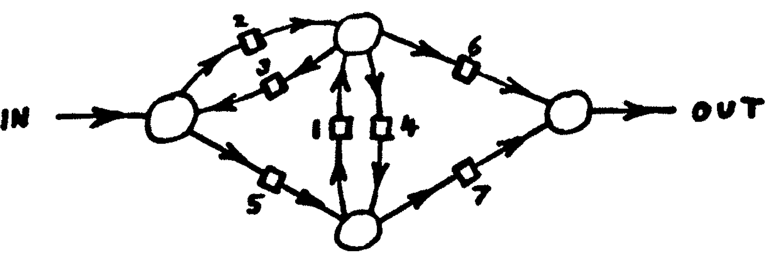
Turing’s illustration of an “unorganized machine” (or neural network) from “Intelligent Machinery,” 1948
Turing and von Neumann were both aware that computing could be done by other means, though. Turing’s model of morphogenesis was a biologically inspired form of massively parallel, distributed computation. So was his earlier concept of an “unorganized machine,” a randomly connected neural net modeled after an infant’s brain. 29 These were visions of what computing without a central processor could look like—and what it does look like, in living systems.
Von Neumann also began exploring massively parallel approaches to computation as far back as the 1940s. In discussions with Polish mathematician Stanisław Ulam at Los Alamos, he conceived the idea of “cellular automata,” pixel-like grids of simple computational units, all obeying the same rule, and all altering their states simultaneously by communicating only with their immediate neighbors. With characteristic bravura, von Neumann went so far as to design, on paper, the key components of a self-reproducing cellular automaton, including a horizontal line of cells comprising a “tape” and blocks of cellular “circuitry” implementing machines A and B.
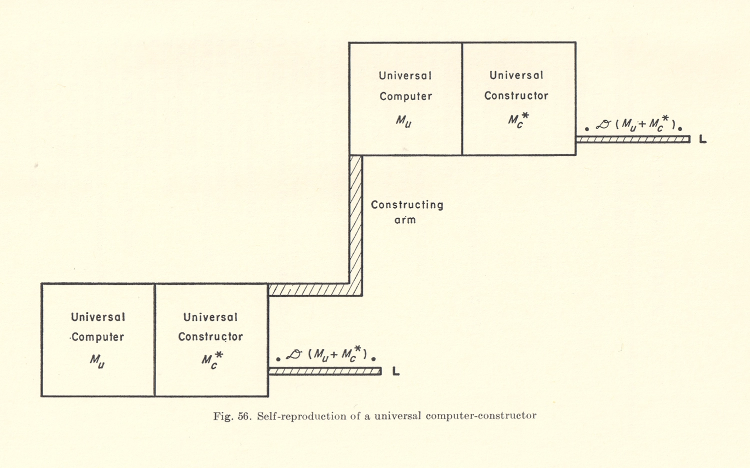
Von Neumann’s universal constructor arm from Theory of Self-Reproducing Automata, 1967
Designing a cellular automaton is far harder than ordinary programming, because every cell or “pixel” is simultaneously altering its own state and its environment. When that kind of parallelism operates on many scales at once, and is combined with randomness and subtle feedback effects, as in biological computation, it becomes even harder to reason about, “program,” or “debug.”
Nonetheless, we should keep in mind what these two pioneers understood so clearly: computing doesn’t have to be done with a central processor, logic gates, binary arithmetic, or sequential programs. One can compute in infinitely many ways. Turing and his successors have shown that they are all equivalent, one of the greatest accomplishments of theoretical computer science.
This “platform independence” or “multiple realizability” means that any computer can emulate any other one. If the computers are of different designs, though, the emulation may run s … l … o … w … l … y. For instance, von Neumann’s self-reproducing cellular automaton has never been physically built—though that would be fun to see! It was only emulated for the first time in 1994, nearly half a century after he designed it. 30
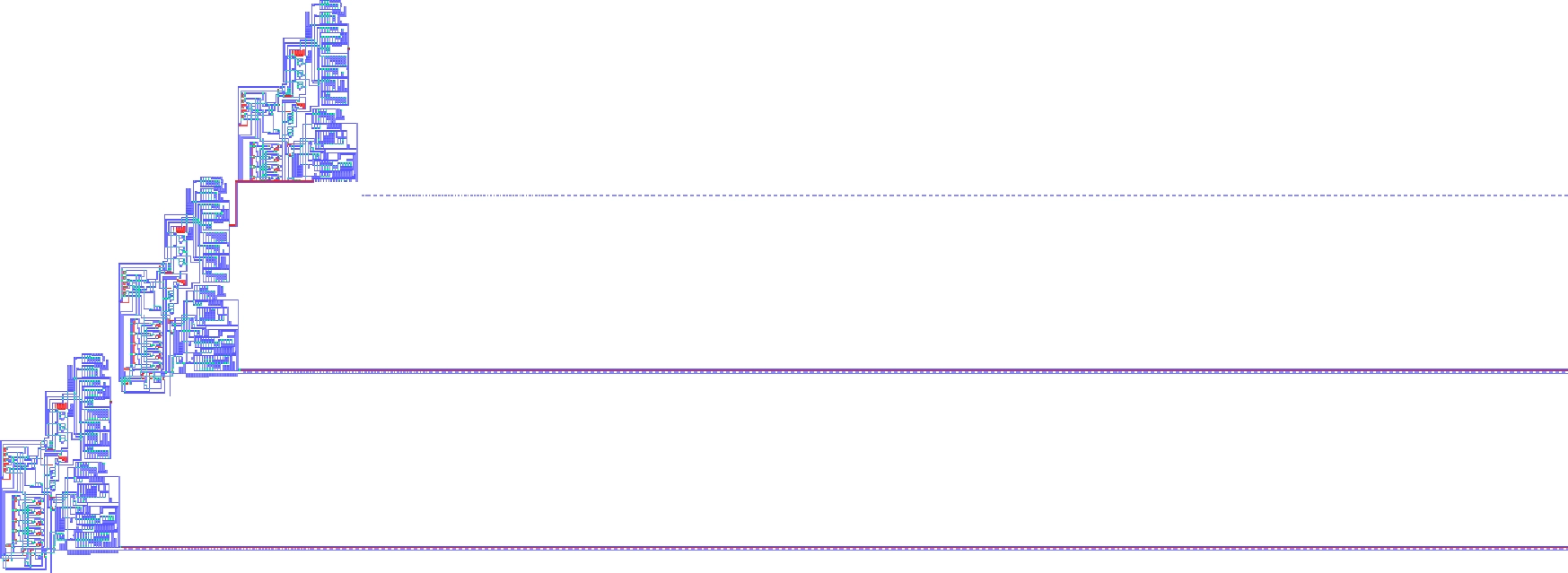
Implementation of von Neumann’s self-reproducing cellular automaton, Pesavento 1995. The second generation has nearly finished constructing the third (lines running off to the right are instruction tapes, much longer than shown).
It couldn’t have happened much earlier. A serial computer requires serious processing power to loop through the automaton’s 6,329 cells over the sixty-three billion time steps required for the automaton to complete its reproductive cycle. Onscreen, it worked as advertised: a pixelated two-dimensional Rube Goldberg machine, squatting astride a 145,315 cell–long instruction tape trailing off to the right, pumping information out of the tape and reaching out with a “writing arm” to slowly print a working clone of itself just above and to the right of the original.
It’s similarly inefficient for a serial computer to emulate a parallel neural network, heir to Turing’s “unorganized machine.” Consequently, running big neural nets like those in Transformer-based chatbots has only recently become practical, thanks to ongoing progress in the miniaturization, speed, and parallelism of digital computers.
In 2020, my colleague Alex Mordvintsev devised a clever combination of modern neural nets, Turing’s morphogenesis, and von Neumann’s cellular automata. Alex’s creation, the “neural cellular automaton” (NCA), replaces the simple per-pixel rule of a classic cellular automaton with a neural net. 31 This net, capable of sensing and affecting a few values representing local morphogen concentrations, can be trained to “grow” any desired pattern or image, not just zebra stripes or leopard spots.
A neural cellular automaton that generates (or re-generates) a lizard emoji, from Mordvintsev et al. 2020
Real cells don’t literally have neural nets inside them, but they do run highly evolved, nonlinear, and purposive “programs” to decide on the actions they will take in the world, given external stimulus and an internal state. NCAs offer a general way to model the range of possible behaviors of cells whose actions don’t involve movement, but only changes of state (here, represented as color) and the absorption or release of chemicals.
The first NCA Alex showed me was of a lizard emoji, which could regenerate not only its tail, but also its limbs and head! It was a powerful demonstration of how complex multicellular life can “think locally” yet “act globally,” even when each cell (or pixel) is running the same program—just as each of your cells is running the same DNA.
This was our first foray into the field known today as “artificial life” or “ALife.”
Artificial Life
Von Neumann’s work on self-reproducing automata shows us that, in a universe whose physical laws do not allow for computation, it would be impossible for life to evolve. Luckily, the physics of our universe do allow for computation, as proven by the fact that we can build computers—and that we’re here at all.
Now we’re in a position to ask: in a universe capable of computation, how often will life arise? Clearly, it happened here. Was it a miracle, an inevitability, or somewhere in between?
A few collaborators and I set out to explore this question in late 2023. 32 Our first experiments used an esoteric programming language invented thirty years earlier by a Swiss physics student and amateur juggler, Urban Müller. I’m afraid he called this language … Brainfuck. Please direct all naming feedback his way.
However, the shoe fits; it is a beast to program in. Here, for instance, is a Brainfuck program that prints “helloworld”—and good luck making any sense of it: ++++++[−>+++++<]>−[>[++++>]++++[<]>−]>>>>.>+.<<…<−.<+++.>.+++.>.>>−. The upside of Brainfuck is its utter minimalism. It’s not quite a single-instruction language, like SUBLEQ, but as you can see, it includes only a handful of operations. Like a Turing Machine, it specifies a read/write head that can step left (the “<” instruction) or right (the “>” instruction) along a tape. The “+” and “−” instructions increment and decrement the byte at the current position on the tape. 33 The “,” and “.” instructions input a byte from the console, or output a byte to it (you can count ten “.” instructions in the code above, one to print each letter of “helloworld”). Finally, the “[” and “]” instructions implement looping: “[” will skip forward to its matching “]” if the byte at the current position is zero, and “]” will jump back to its matching “[” if the byte is nonzero. That’s it!
It’s hard to believe that Brainfuck could be used to fully implement, say, the Windows operating system, but it is “Turing complete.” Here that means: given enough time and memory (that is, a long enough tape), it can emulate any other computer and compute anything that can be computed.
In our version, which we call bff, there’s a “soup” containing thousands of tapes, each of which includes both code and data. This is key: in “classic” Brainfuck, the code is separate from the tape, whereas in bff, we wanted the code to be able to modify itself. That can only happen if the code itself is on the tape, as Turing originally envisioned.
Bff tapes are of fixed length—64 bytes, about the same length as the cryptic “helloworld” program above. They start off filled with random bytes. Then, they interact at random, over and over. In an interaction, two randomly selected tapes are stuck end to end, and this combined 128 byte–long tape is run, potentially modifying itself. The 64 byte–long halves are then pulled back apart and returned to the soup. Once in a while, a byte value is randomized, as cosmic rays do to DNA.
Since bff has only seven instructions (represented by the characters “<>+−,[]”) and there are 256 possible byte values, following random initialization only 7/256, or 2.7 percent, of the bytes in a given tape will contain valid instructions; any non-instructions are simply skipped over. 34 Thus, at first, not much comes of interactions between tapes. Once in a while, a valid instruction will modify a byte, and this modification will persist in the soup. On average, though, only a couple of computational operations take place per interaction, and usually, they have no effect. In other words, while any kind of computation is theoretically possible in this toy universe, precious little actually takes place—at first. Random mutation may alter a byte here and there. Even when a valid instruction causes a byte to change, though, the alteration is arbitrary and purposeless.
But after millions of interactions, something magical happens: the tapes begin to reproduce! As they spawn copies of themselves and each other, randomness gives way to intricate order. The suddenness of this change resembles a “phase transition” in matter, as between gas and liquid, or liquid and solid. Indeed, the initial disorder of the soup is very much like that of randomly whizzing gas molecules. Hence random, non-functional code has been called “Turing gas”; 35 however, in bff, it “condenses” into functioning code, which is something far more complex than a solid or a liquid.
An early run of bff showing evolution from random initialization to full-tape replication; only bytes coding for instructions are shown.
We could call it “computronium,” 36 since when the phase transition occurs, the amount of computation taking place skyrockets—remember, reproduction requires computation. Two of Brainfuck’s seven instructions (“[” and “]”) are dedicated to conditional branching, and define loops in the code. Reproduction requires at least one such loop (“copy bytes until done”), causing the number of instructions executed in an interaction to climb into the thousands.
Scatter plot showing the first thirty million interactions in a bff run as dots with height equal to the number of operations. Note the sharp transition to computing-intensive full-tape replication at fifteen million interactions.
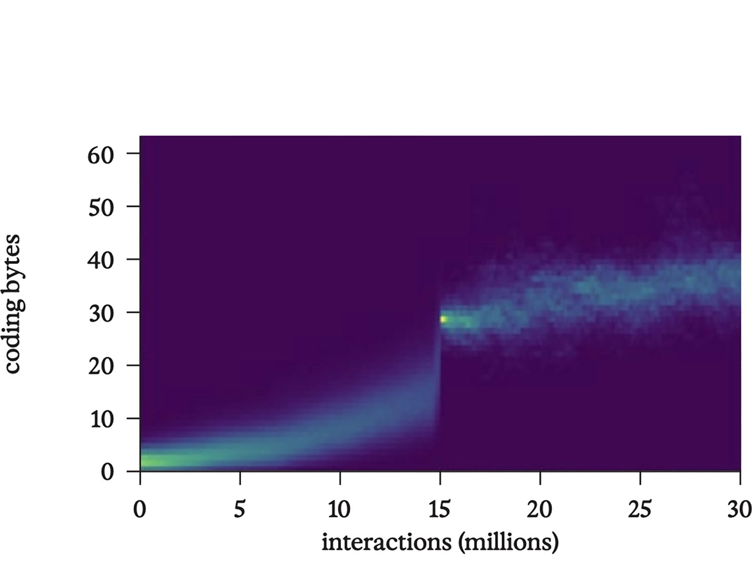
Histogram showing number of bytes coding for instructions per tape in the same bff run; note the ongoing rise in the amount of code even after the transition to full-tape replication at fifteen million interactions.
The code is no longer random, but obviously purposive, in the sense that its function can be analyzed and reverse-engineered. An unlucky mutation can break it, rendering it unable to reproduce. Over time, the code evolves clever strategies to increase its robustness to such damage.
This emergence of function and purpose is just like what we see in organic life at every scale; so we can talk about the function of the circulatory system, a kidney, or a mitochondrion, and how they can “fail”—even though nobody designed these systems.
We reproduced our basic result with a variety of other programming languages and environments. Alex (of neural cellular automata renown) created another beautiful mashup, this time between cellular automata and bff. Each of a 200×200 array of “pixels” contains a program tape, and interactions occur only between neighboring tapes on the grid. In a nod to our nerdy childhoods, the tapes are interpreted as instructions for the iconic Zilog Z80 microprocessor, launched in 1976 and used in many 8-bit computers over the years (including the Sinclair ZX Spectrum, Osborne 1, and TRS-80). Here, too, complex replicators soon emerge from random interactions, evolving and spreading across the grid in successive waves.
Evolution of competing replicators on a 200×200 grid of simulated Zilog Z80 processors
Our simulations suggest that, in general, life arises spontaneously whenever conditions permit. Those conditions seem minimal: little more than an environment capable of supporting computation, some randomness, and enough time.
Let’s pause and take stock of why this is so remarkable.
On an intuitive level, one does not expect function or purposiveness to emerge spontaneously. To be sure, we’ve known for a long time that a modest degree of order can emerge from initially random conditions; for instance, the lapping of waves can approximately sort the sand on a beach, creating a gradient from fine to coarse. But if we were to begin with sand on a beach subject to random wave action, and came back after a few hours to find a poem written there, or the sand grains fused into a complex electronic circuit, we would assume someone was messing with us.
The extreme improbability of complex order arising spontaneously is generally understood to follow from thermodynamics, the branch of physics concerned with the statistical behavior of matter subject to random thermal fluctuations—that is, of all matter, since above absolute zero, everything is subject to such randomness. Matter subject to random forces is supposed to become more random, not less. Yet by growing, reproducing, evolving, and indeed by existing at all, life seems to violate this principle.
The violation is only apparent, for life requires an input of free energy, allowing the forces of entropy to be kept at bay. Still, the seemingly spontaneous emergence and “complexification” of living systems has appeared to be, if not strictly disallowed by physical laws, at least unexplained by them. That’s why the great physicist Erwin Schrödinger (1887–1961) wrote, in an influential little book he published in 1944 entitled What Is Life?,
[L]iving matter, while not eluding the “laws of physics” as established up to date, is likely to involve “other laws of physics” hitherto unknown, which, however, once they have been revealed, will form just as integral a part of this science as the former. 37
Thermodynamics
Before turning to those “other laws of physics,” it’s helpful to take a closer look at the original ones, and especially the Second Law of thermodynamics.
These are deep waters. While the fundamental ideas date back to the groundbreaking work of nineteenth-century mathematical physicist Ludwig Boltzmann (1844–1906), we can understand their essence without math. Nonetheless, Boltzmann’s conceptually challenging ideas flummoxed many of his fellow scientists, and the implications of his work continue to stir controversy even today. Much has been made of Einstein turning our everyday notions of space and time inside-out with his theory of relativity, developed in its initial form in 1905—just a year before Boltzmann, struggling with bipolar disorder, ended his own life. Arguably, though, Boltzmann’s earlier ideas disrupt our intuitions about time, cause, and effect even more radically than Einstein’s theory of relativity. 38 Let’s dive in.

Rusted and pitted struts of the partially collapsed seventy-year-old Nandu River Iron Bridge, Hainan Province, China
The Second Law of thermodynamics holds that any closed system will rise in entropy over time, becoming increasingly disordered. A hand-powered lawn mower, for example, starts off as a beautifully polished machine with sharp helical blades, round wheels, and toothed gears, all coupled together on smoothly rotating bearings. If left out in the elements, the bearings will seize up, the blades will dull, and oxidation will set in. After enough time, only a heap of rust will remain.
Similarly, if you were to take a dead bacterium (which, though a lot smaller, is far more complicated than a push mower) and drop it into a beaker of water, its cell membrane would eventually degrade, its various parts would spill out, and after a while only simple molecules would remain, dispersed uniformly throughout the beaker.
The Second Law gives time its arrow, because the fundamental laws of physics in our universe are very nearly time-reversible. 39 Strange, but true: Newton’s equations (classical dynamics), Maxwell’s equations (electromagnetism), Schrödinger’s equations (quantum physics), Einstein’s equations (special and general relativity)—all of these physical laws would work the same way if time ran in reverse. The difference between past and future evaporates when we look only at the mathematics of dynamical laws, or only at an individual microscopic event in the universe. The distinction between past and future, or cause and effect, only comes into view when we zoom out from that microscopic world of individual events and consider instead their statistics.
Here’s a common undergraduate thought experiment to illustrate this point in the case of Newtonian dynamics. Imagine video footage of balls on a billiard table, all in random positions and moving in random directions. They will collide with one another and with the bumpers at the edge of the table, bouncing off at new angles. If we (unrealistically) assume frictionless motion and fully elastic collisions (i.e., balls don’t slow down as they roll, and none of the collision energy is dissipated as heat), this would go on forever. The summed momenta and summed energies of the balls will remain constant—and it will be impossible to tell whether you’re watching the video forward or in reverse. In such a universe, causality has no meaning, because nothing distinguishes causes from effects.
If the initial conditions were random, then the positions of the balls will continue to be randomly distributed over the table’s surface as they all bounce around, transferring some of their energy to each other with every collision. It would be astronomically unlikely for the balls to all bunch up in one spot. Their velocities, too, will be randomly distributed, both in direction and magnitude, so it would also be astronomically unlikely for them to, for instance, suddenly all be moving precisely parallel to the table’s edges. Complete disorder, in other words, is a stable equilibrium. 40 In the presence of any thermal noise (that is, random perturbation), it is the only stable equilibrium.
Suppose, though, that the near-impossible happens. You see fifteen of the balls converge into a perfect, stock-still triangular grid, each ball just touching its neighbors, while the cue ball, having absorbed all of the combined kinetic energy of the other fifteen, whizzes away from the triangle. Aha! Now, we know that we’re watching a pool break—and we know that we’re watching it in reverse. The arrow of time has been established. Along with it, we have causation: the triangle broke because it was hit by the cue ball.
Billiard balls in motion: forward or backward in time?
Theoretically, nothing prevents the exact series of collisions from happening that would result in all of the energy being transferred to a single ball while leaving the others arrayed in a perfect triangle; but statistically, it’s vanishingly unlikely for such an ordered state to arise out of disorder—unless, perhaps, some mastermind set the balls in motion just so.
Although key thermodynamic concepts were not developed until the nineteenth century, an Enlightenment-era belief in a God who set the universe in motion just so arises intuitively from the apparent impossibility of order arising spontaneously out of disorder. 41 In a mechanical, billiard-table universe where the laws of physics are inviolable and the laws of statistics seem to inexorably degrade any pre-existing order over time, it seems absurd that anything as complicated as life could arise spontaneously without some supernatural agent acting as “prime mover.” Only a God with exquisite foresight could have “initialized” the Big Bang such that, in the Earth’s oceans billions of years ago, simple organic molecules floating around apparently at random could coalesce into a working bacterium—an improbability many, many orders of magnitude less likely than fifteen out of sixteen whizzing billiard balls spontaneously coalescing into an unmoving triangle.
The billiard ball universe I’ve just described may seem abstract or arbitrary, but nineteenth-century theorists like Boltzmann had become interested in this problem for the most practical of reasons: it was the physics behind steam power, hence the entire Industrial Revolution. 42 Engineering had preceded theory, as it often does.
Thomas Newcomen (1664–1729), an English inventor and Baptist lay preacher, devised the first practical fuel-burning engine in 1712. It was based on a heating-and-cooling cycle. First, steam from a boiler was allowed to flow into a cylindrical chamber, raising a piston; then, the steam valve closed, and a second valve opened, injecting a jet of cold water, causing the steam to condense and pull the piston back down. As the piston rose and fell, it rocked a giant beam back and forth, which, in Newcomen’s original design, was used to pump water out of flooded mines (which, in turn, supplied the coal these engines would soon be consuming so voraciously).
Scottish inventor and entrepreneur James Watt (1736–1819) greatly improved the steam-engine design in 1776, making it a practical replacement for human and animal power across a wide range of applications. This was when the Industrial Revolution really got underway; for the first time, human-made machines began to metabolize on a large scale, “eating” complex organic molecules to perform mechanical work.
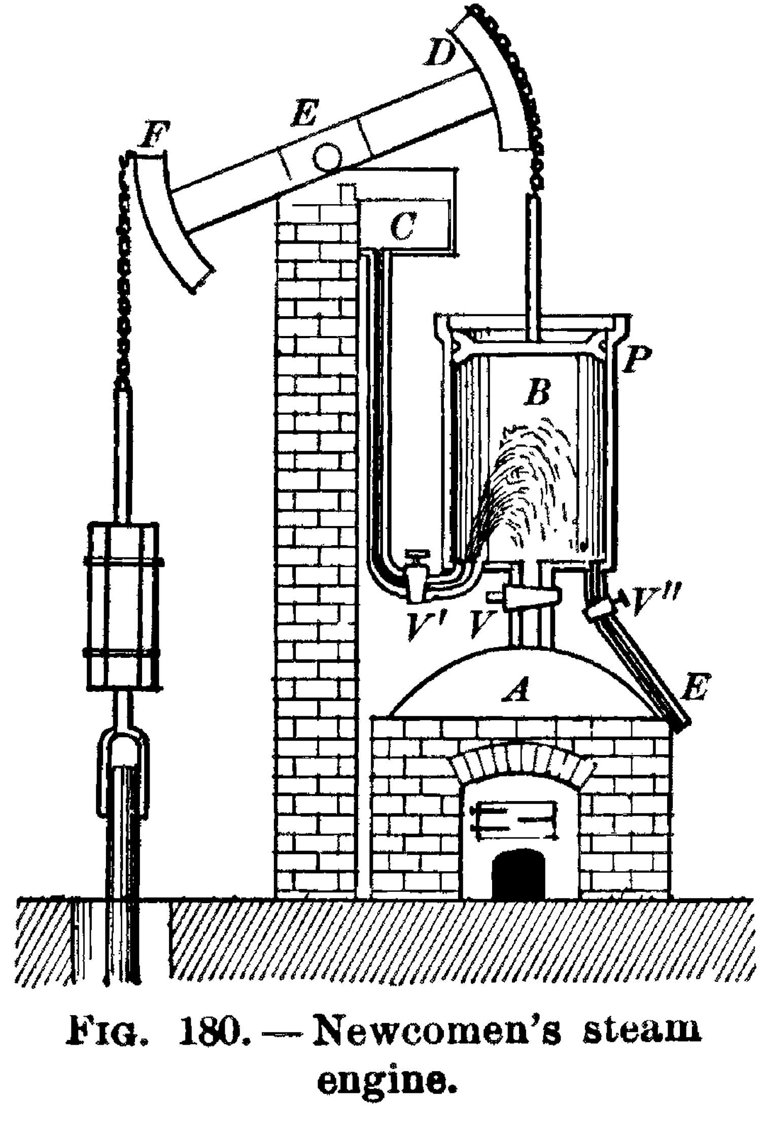
Newcomen’s steam engine, from Black and Davis, Practical Physics, 1913
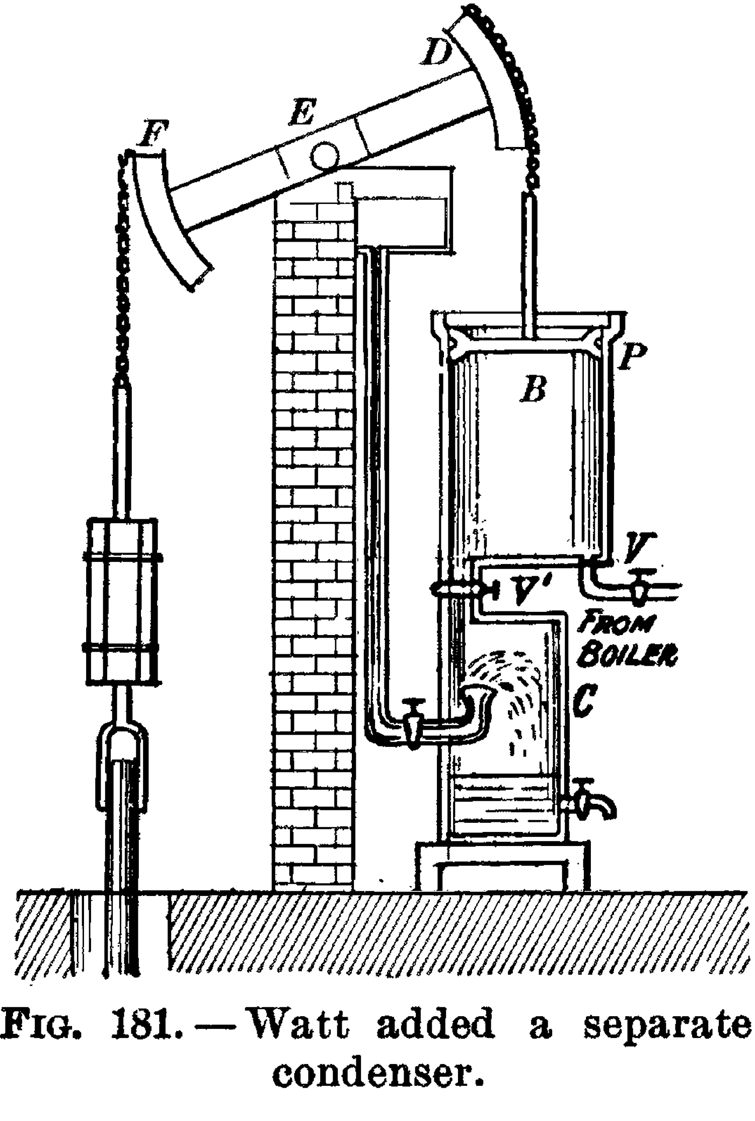
Watt’s steam engine, ibid.
Soon, far more energy would be flowing through this artificial metabolism than through the Krebs cycle in our own bodies. 43 It was, in the broad sense I’ve been using in this book, a major evolutionary transition: a symbiogenetic event between humans and machines, like earlier symbioses between humans and draft animals. Machine metabolism allowed human society to explode from its pre-industrial scale (about one billion people in 1800, most of whom lived in extreme poverty) to its scale today (eight billion, most of whom no longer live in poverty). 44 In the process, we’ve become nearly as dependent on machines for our continued existence as they are on us.
However, even as coal-powered engines transformed the Victorian landscape—both figuratively and literally, for the pollution was dire—nobody understood them at a deep level. What was heat, and how could it be converted into physical work? For a time, the leading theory held that heat was a kind of invisible, weightless fluid, “caloric,” that could flow spookily into and through other matter.
By combining Newtonian physics, statistical calculations, and experimental tests, Boltzmann and his colleagues figured out what was really going on. Their conceptual setup was a three-dimensional version of the billiard table, in which the balls were gas molecules whizzing around in a pressurized chamber, bouncing off its walls. Calculating the average effect of all the bouncing led to the Ideal Gas Law, which established theoretical relationships between the pressure, volume, and temperature of a gas. The theory closely matched observations by experimentalists and engineers. 45
Volume is straightforward (that’s just the size of the chamber), but the idea that pressure is the aggregate force on the chamber’s walls as molecules bounce off them, and that temperature is the average kinetic energy 46 of those whizzing molecules, was a profound insight. There was no need for any mysterious “caloric” fluid; heat was just motion on a microscopic scale. And the tendency toward a random distribution of molecular positions and momenta explains why, if you open a valve between two chambers containing gas at different pressures and/or temperatures, those pressures and temperatures will quickly equalize.
Before moving beyond classical thermodynamics, let’s add a bit more realism to our billiard-ball universe. We know that balls bouncing around a billiard table don’t actually go on bouncing forever. They encounter friction, slowing down as they roll. And when they bounce off each other, the collisions are slightly “inelastic,” meaning that after the collision, they’re moving a bit slower than before. After a little while, they stop rolling.
How can that be? At a microscopic level, the laws of physics are reversible. Momentum is supposed to be conserved. And the amount of matter and energy also remains constant, whether we run time forward or in reverse. That’s the First Law of thermodynamics!
Zooming in will reveal that, on a real billiard table, balls aren’t the smallest elements that bump against one other. Each billiard ball consists of lots of vibrating molecules bound together. Collisions between these individual molecules are what really cause the balls to bounce off each other—or, for that matter, cause a ball to roll across the felt rather than falling right through it. 47 In each case, momentum is transferred between molecules. Every time this happens, the distribution of molecular momenta becomes a bit more random, that is, a bit less correlated with which ball the molecule happens to be in, or indeed whether it is in a ball at all, or in the felt underneath.
In the most random distribution of molecular velocities, there would be no more correlation between the velocities of two molecules in one ball than in the velocities of molecules in different balls. Every ball would be imperceptibly jiggling in place, with each of its constituent molecules contributing minutely to the dance. We call that random jiggling “heat.” When all correlated motion has been converted into uniformly distributed heat, we’ve reached a stable equilibrium.
While the balls are still rolling, the correlations between the velocities of their molecules are by no means all equal; the distribution is far from random. This is not a stable equilibrium. Hence, the inevitability of friction and the inelasticity of collisions are statistical phenomena—just more symptoms of the inexorable Second Law.
Going forward, then, let’s imagine once more that the billiard balls are indivisible particles, not bound collections of molecules. In that case, all collisions would have to be elastic, all motion frictionless, and disordered, randomly colliding balls would be the equilibrium.
Once a system has reached equilibrium, it will stay that way forever—an end state Lord Kelvin called “heat death.” 48 This seemingly trivial observation has some profound consequences. First, the arrow of time will lose its meaning; any two consecutive moments A, B could just as likely have been ordered B, A. Nothing, therefore, can be said to be a cause, versus an effect.
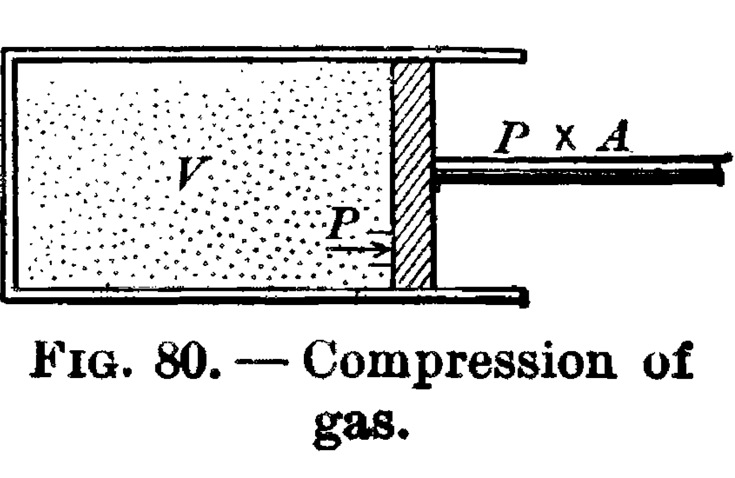
A piston with a face of area A and interior volume V containing an ideal gas at pressure P, ibid.
Relatedly, no work can be done. If the system were out of equilibrium—for instance, if all of the whizzing balls were on one side of the billiard table—then we could put a movable barrier down between the empty and occupied sides, attached to a loaded crankshaft. As they bounce around, the balls would then nudge the barrier, doing work. What I’ve just described is, of course, a piston, like that of a steam engine.
But if the balls were equally likely to be anywhere, then no matter how fast they whizz and bounce, there’s nowhere to put the barrier that would result in any net force. The piston wouldn’t move because it would be buffeted equally from all sides. This idea can be generalized: work can only be done by a system in disequilibrium, for instance, when the pressure or temperature is high in one place, and low in another. That’s why Newcomen’s engine needed both hot steam and cold water.
I’ve already used the term free energy, but now we can define it. The free energy of a system is the amount of work it can be made to do. Far from equilibrium, when the entropy is low, much of the kinetic energy in the billiard balls is “free”; it can be used to move pistons, raise weights, produce electric currents, carry out computations, or drive metabolic processes. But at equilibrium, the entropy is maximized, and the free energy is zero. This insight into the relationship between energy, entropy, and work lies at the heart of thermodynamics—and life.
Dynamic Stability
Recall that life seemed deeply weird to Schrödinger because living things appear to violate the Second Law. If the bacterium we drop into a beaker of water is alive rather than dead, and free energy is available in a form the bacterium can use, and the water contains simple molecules suitable for building more bacteria, then over time we will see the very opposite of an increase in disorder. After a while, the beaker will be full of bacteria, reproducing, cooperating, and competing with each other.
The bacteria will even be evolving. If the beaker is sufficiently large—the size of a planet, for instance—and we wait a few billion years, then eventually beings as complicated as us may be in there, along with cities, advanced technologies, and perhaps plans to colonize a nearby beaker.
None of these processes can occur without free energy. For us, it comes primarily from the sun. Thermodynamics tells us that even if the Second Law appears to be violated locally, it still holds when we zoom out. Order created in one place comes at the expense of increased disorder elsewhere. Hence, pollution, the finite lifetime of the sun, and the eventual heat death of the universe.
What concerns us here isn’t this big picture, but its apparent local violations, and the way they seem to become increasingly transgressive over time. The puzzle isn’t only that bacteria exist, but that as time passes, life on Earth seems to become more complex: from prokaryotes to eukaryotes; from eukaryotes to multicellular animals; from simple multicellular animals to ones with nervous systems; from brainy animals to complex societies; from horses and plows to space travel and AI.
Is there any general principle behind that complexification process, a kind of “however” or “yes, and” to the dismal Second Law? And could it account not only for evolution and complexification, but also for abiogenesis?
Yes, and yes. Bff can offer us a highly simplified model system for understanding that principle, just as an idealized billiard table gives us a model for understanding basic thermodynamics.
Replicators arise in bff because an entity that reproduces is more “dynamically stable” than one that doesn’t. In other words, if we start with one tape that can reproduce and one that can’t, then at some later time we’re likely to find many copies of the one that can reproduce, but we’re unlikely to find the other at all, because it will have been degraded by noise or overwritten.
Addy Pross, a professor emeritus of chemistry at Ben Gurion University of the Negev, describes the same phenomenon using the bulkier phrase “dynamic kinetic stability” (DKS). 49 I’ll drop “kinetic,” since the idea also applies far beyond Pross’s field of “chemical kinetics” (describing the rates at which chemical reactions take place). In bff, for example, dynamic stability can just as well apply to programs or program fragments.
As Pross points out, a population of replicating molecules can be more stable than even the hardiest of passive materials. A passive object may be fragile, like a soap bubble, or robust, like a stone sculpture. The sculpture might endure for longer, but, in the end, it’s still ephemeral. Every encounter it has with anything else in the world will cause its composition or structure to degrade, its individual identity to blur. For a sculpture, it’s all downhill. That’s the Second Law at work, as usual.
A self-reproducing molecule—like the DNA inside a living bacterium—is another matter. It is thermodynamically fragile, especially if we consider its identity to consist not only of a general structure but of a long sequence of specific nucleotides. However, its pattern is not just robust, but “antifragile.” 50 As long as DNA is able to reproduce—an inherently dynamic process—that pattern can last, essentially, forever. A bit of environmental stress or adversity can even help DNA maintain or improve its functionality. 51 This is how order overcomes disorder.
In fact, Darwinian selection is equivalent to the Second Law, once we expand our notion of stability to include populations of replicators. Through a thermodynamic lens, Darwin’s central observation was that a more effective replicator is more stable than a less effective one. As Pross puts it,
[M]atter […] tends to become transformed […] from less stable to more stable forms. […] [T]hat is what chemical kinetics and thermodynamics is all about […]. And what is the central law that governs such transformations? The Second Law. […] In both [the static and kinetic] worlds chemical systems tend to become transformed into more stable ones […]—thermodynamic stability in the “regular” chemical world, dynamic kinetic stability in the replicator world. 52
As a chemist, Pross is sensitive to the close relationships between energy, entropy, and stability, whether static or dynamic. However, he does not explicitly make a connection to the theory of computing.
It now seems clear that by unifying thermodynamics with the theory of computation, we should be able to understand life as the predictable outcome of a statistical process, rather than regarding it uneasily as technically permitted, yet mysterious. Our artificial life experiments demonstrate that, when computation is possible, it will be a “dynamical attractor,” since replicating entities are more dynamically stable than non-replicating ones; and, as von Neumann showed, replicators are inherently computational.
Bff has no concept of energy, but in our universe, replicators require an energy source. This is because, in general, computation involves irreversible steps—otherwise known as causes and effects—and thus, computing consumes free energy. That’s why the chips in our computers draw power and generate heat when they run. (And why my computer heats up when it runs bff.) Life must draw power and generate heat for the same reason: it is inherently computational.
Complexification
When we pick a tape out of the bff soup after millions of interactions, once replicators have taken over, we often see a level of complexity in the program on that tape that seems unnecessarily—even implausibly—high. A working replicator could consist of just a handful of instructions in a single loop, requiring a couple of hundred operations to run. Instead, we often see instructions filling up a majority of the 64 bytes, multiple and complex nested loops, and thousands of operations per interaction.
Where did all this complexity come from? It certainly doesn’t look like the result of simple Darwinian selection operating on the random text generated by a proverbial million monkeys typing on a million typewriters. 53 In fact, such complexity emerges even with zero random mutation—that is, given only the initial randomness in the soup, which works out to fewer bytes than the text of this book. Hardly a million monkeys—and far too few random bytes to contain more than a few consecutive instructions, let alone a whole working program.
The answer recalls Lynn Margulis’s great insight: the central role of symbiosis in evolution, rather than random mutation and selection. When we look carefully at the quiescent period in the bff soup before tapes begin replicating, we notice a steady rise in the amount of computation taking place. We are observing the rapid emergence of imperfect replicators—very short bits of code that, in one way or another, have some nonzero probability of generating more code. Even if the code produced is not like the original, it’s still code, and only code can produce more code; non-code can’t produce anything!
Thus, a selection process, wherein code begets code, is at work from the very beginning. This inherently creative, self-catalyzing process is far more important than random mutation in generating novelty. When bits of proliferating code combine to form a replicator, it’s a symbiotic event: by working together, these bits of code generate more code than they could separately, and the code they generate will in turn produce more code that does the same, eventually leading to whole-tape replication and an exponential takeoff.
A closer look at the bff soup prior to the exponential takeoff reveals distinct phases of “pre-life,” which might have had close analogs during abiogenesis on Earth. In the first phase, individual instructions occasionally generate another individual instruction, but this is more akin to a simple chemical reaction than to any real computation; the instructions are not acting as part of any larger program.
In the second phase, we begin to see instructions in particular positions, or in particular combinations, that are likelier to lead to copies of themselves than one would expect by random chance, albeit often in indirect ways. “Autocatalytic sets” start to form: cycles of dynamical interactions that mutually reinforce each other. These, too, can arise spontaneously in the chemical world, and have long been theorized to have driven abiogenesis. 54
At this point, with autocatalytic fragments of code proliferating and colliding, a leap becomes possible that brings us beyond the world of digital chemistry and into the world of real computation: the emergence of the first true replicators. These are no longer mere autocatalytic sets, but short programs that copy themselves, or each other, using looped instructions.
With this leap to computation comes an enormous upgrade in evolvability, because now, any change made to a program that does not break its copy loop will be heritable. Thus, classical Darwinian selection can kick in, allowing adaptation to a changing environment or speciation for occupying diverse niches. If we insist on making a distinction between non-life and life, this might be a reasonable place to draw that line.
However, these earliest replicating programs are unlikely to cleanly copy a whole tape. Often, they only copy short stretches of tape, which may get pasted into arbitrary locations, yielding unpredictable results. As these scrappy, fragmentary replicators proliferate, the bff soup enters a chaotic phase. Despite the churn, the tapes have not, at this point, resolved into any obvious structure. To the naked eye, they still look like random junk, although the rising amount of computation taking place (as measured both by the average number of operations per interaction and the density of instructions per tape) suggests that something is afoot.
Tracking the provenance of every byte in the soup, starting from random initialization, can make sense of the apparent chaos. At first, almost every byte of every tape remains whatever it was at initialization time; if we draw a line from each byte’s current position on a tape to its original source position, the lines will all extend back to time zero in parallel, like the warp threads of a loom. Once in a while, a byte will change, cutting a thread, or get copied, pulling it across the other threads diagonally.
Provenance of individual bytes on tapes in a bff soup after 10,000, 500,000, 1.5 million, 2.5 million, 3.5 million, 6 million, 7 million, and 10 million interactions. The increasing role of self-modification in generating novelty is evident, culminating in the emergence (just before 6 million interactions) of a full-tape replicator whose parts are modified copies of a shorter imperfect replicator.
With the rise of scrappy replicating programs, all remaining dependencies on the past are quickly cut as replicators copy over each other in a frenzy of creative destruction. Any given byte might get copied hundreds of times to a series of different tape locations, in the process wiping out whatever had previously been there. Shortly afterward, all of those copies might get wiped out in turn by some other more efficiently replicating fragment. Soon, every byte’s history becomes very brief in time, yet complex in space—a short-lived snarl of sideways jumps. The loom becomes all weft, and no warp.
Are these scrappy replicators competing or cooperating? Both. Replicators that can’t keep up are wiped out, along with any non-replicating bytes. Surviving replicators, on the other hand, continually form chimeras, 55 recombining with other replicators (or even copies of themselves) to become more effective still. These are, once more, symbiogenetic events: sub-entities merging to form a larger, more capable super-entity.
This chaotic phase is such a potent crucible for directed evolution that it generally doesn’t last long. It rapidly produces a robust whole-tape replicator, which then takes off exponentially, resulting in the dramatic transition to the organized structures (and large amounts of computation) that are bff’s most obvious feature. At this point, artificial life seems to spontaneously emerge.
But as we can now appreciate, there’s nothing spontaneous about it. Replicators had been present all along, and each larger replicator is composed of smaller ones—an inverted tree of life, consisting of mergers over time rather than splits.
However, evolution’s creative work is not done yet. After the takeoff of a fully functional tape replicator, we often see yet further symbiotic events. From a classical Darwinian standpoint, this seems puzzling, since further evolution seems superfluous once whole tapes are replicating reliably. How could “fitness” possibly improve further, once a tape copies itself in its entirety every time it interacts with another tape?
We must consider that since the instructions for whole-tape replication don’t occupy all 64 bytes, there’s extra space on the tape that could be dedicated to … anything. That’s the point of von Neumann–style replication—it allows for open-ended evolution precisely because the tape can contain additional information, beyond the code needed for replication itself. 56
Any extra replicated bytes could, of course, be random—just passive, purposeless information cargo hitchhiking from one generation to the next. But if these bytes contain instructions, those instructions can run. And if they can run, they can replicate themselves, too. Thus, the symbiogenetic process can continue to operate, creating additional replicators within an already replicating tape. Sometimes these sub-replicators even produce multiple copies of themselves in a single interaction.
Sub-replicators can interact with their host in many ways. They can “kill” the host by damaging its replication code, which is generally catastrophic for the sub-replicator, as it thereby destroys the environment within which it can run. Sub-replicators can be neutral, leaving the host’s replication machinery alone. Or, they can be symbiotic, for instance by conferring resistance to mutational damage via redundant copying of the host’s code. The overall tendency is toward symbiosis, since that is the most dynamically stable.
Over time, code colonizes a large proportion of the 64 bytes. Code is more dynamically stable than non-code, and its dynamic stability increases through symbiosis with yet more code—in particular, when code fragments find ways to work in functional tandem.
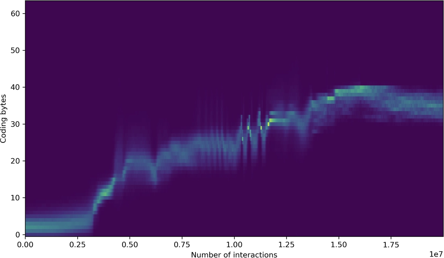
Histogram showing how many of a tape’s 64 bytes code for instructions; note, as before, the ongoing rise after full-tape replication, which here begins at about 3 million interactions.
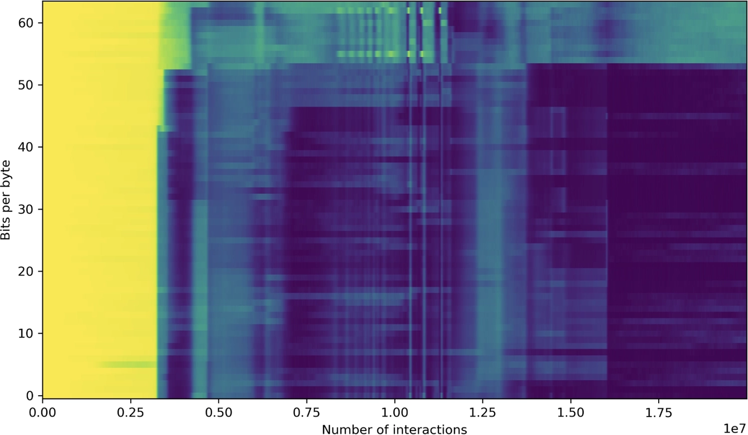
The variability or amount of information in a tape byte at each position, expressed as an entropy in bits. Prior to the transition, the value is close to 8 (corresponding to a random distribution over values 0–255), but at the time of transition to full-tape replication it drops dramatically; some positions are more variable than others, though, with higher variability toward the end of the tape.
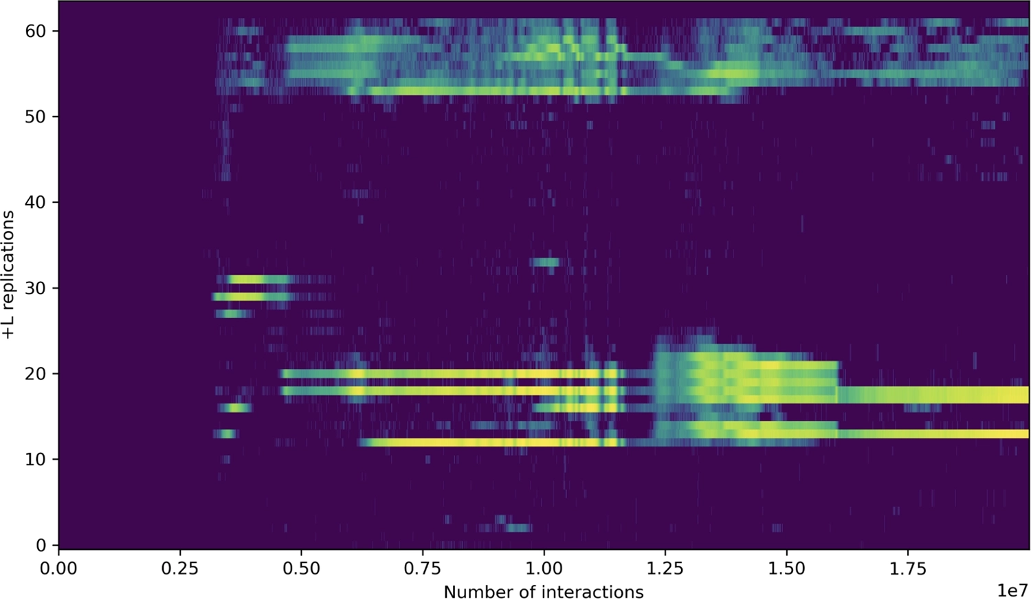
Histogram showing positions of “[” loop instructions that perform an “aligned” copy of a tape region on one tape to the same position on the other tape, corresponding to perfect replication. Note that there are multiple perfect replicators in the soup, with populations that change over time.
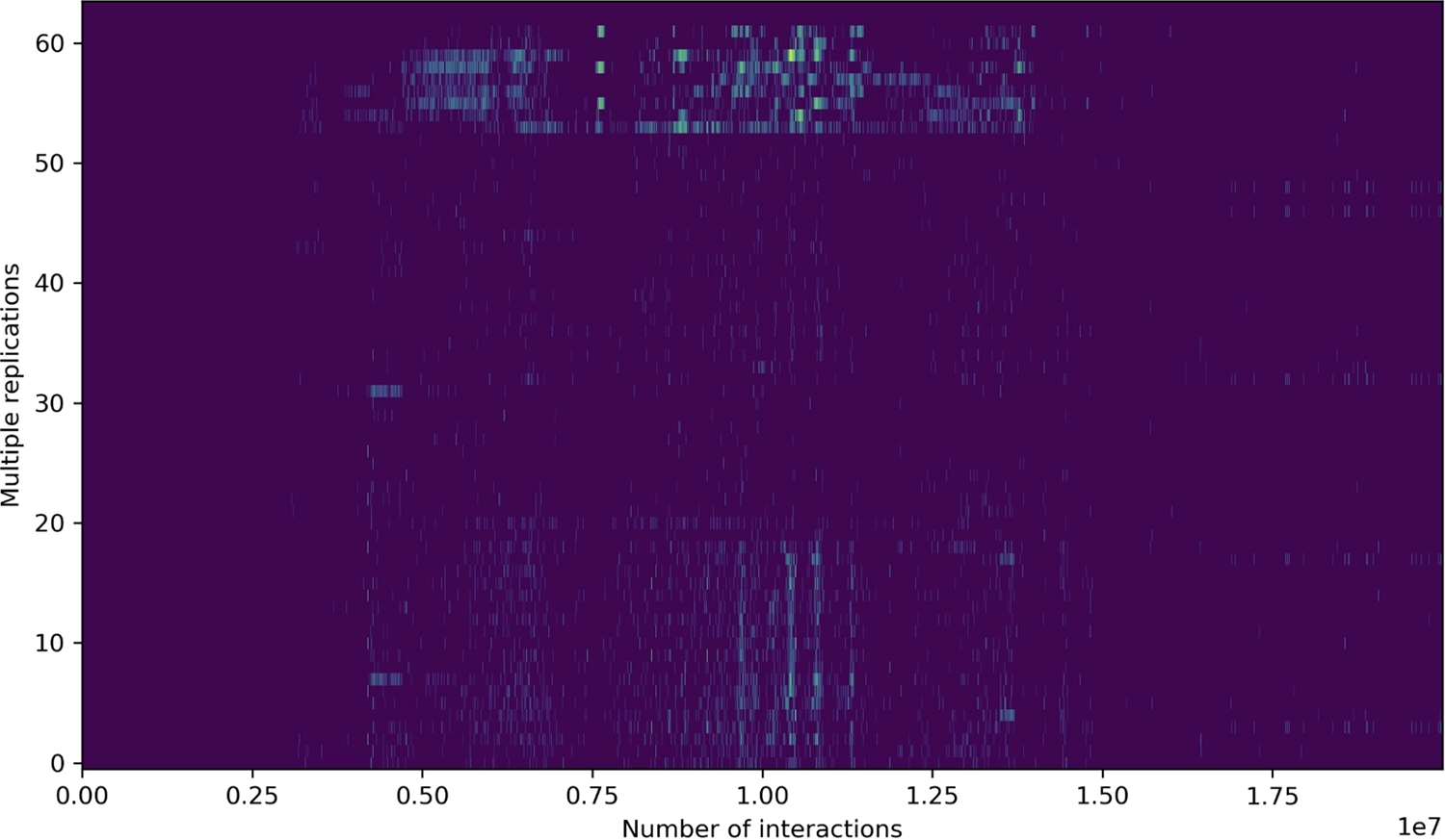
Histogram showing positions of “[” loop instructions that replicate themselves multiple times when run, shown emerging in this run after full-tape replication.
In a way, symbiosis is the very essence of functionality. When we talk about a kidney’s function only making sense in context, we mean that it is in symbiosis with other functions—like those of the liver (breaking ammonia down into urea), the heart (pumping blood), and so on. Each of these functions is purposive precisely because its inputs are the outputs of others, its outputs are inputs to others, and thus they form a network of dynamically stable cycles.
The same is true of larger, planetary-scale interrelationships. The “purpose” of plants, from the perspective of animal life, is to produce oxygen and sugar, which we breathe and eat. The “purpose” of animals, from a plant’s perspective, is to turn the oxygen back into carbon dioxide, and provide compost and pollination. Our growing understanding of life as a self-reinforcing dynamical process boils down not to things, but to networks of mutually beneficial relationships. At every scale, life is an ecology of functions.
Because functions can be expressed computationally, we could even say that life is code. Individual computational instructions are the irreducible quanta of life—the minimal replicating set of entities, however immaterial and abstract they may seem, that come together to form bigger, more stable, and more complex replicators, in ever-ascending symbiotic cascades.
In the toy universe of bff, the seven special characters “<>+−,[]” are the elementary instructions. On the primordial sea floor, geothermally-driven chemical reactions that could catalyze further chemical reactions likely played the same role. Under other conditions, on another planet, or in another universe, many different elementary interactions could do the same—as long as they are Turing complete, enabling them to make the leap from autocatalytic sets to true replication.
Virality
Although bff is only a toy universe, it can serve as a simplified model for life and evolution, just as a Newtonian billiard-ball universe can serve as a simplified model for the thermodynamics of ideal gases. As we’ve seen, some of bff’s predictions are quite different from those of classical Darwinian theory:
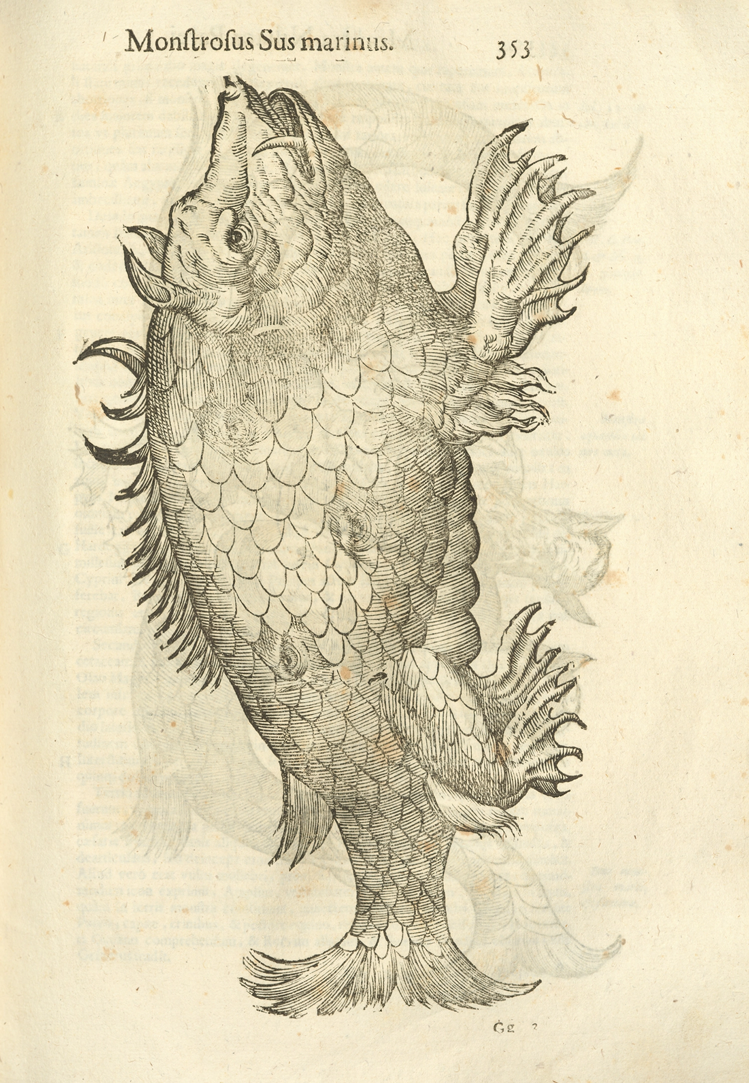
Sea monster from Ulisse Aldrovandi, Monstrorum Historia, 1642
- Bff suggests that symbiogenesis is a more important driver of evolutionary innovation than random mutation.
- Since symbiogenesis must involve combinations of pre-existing dynamically stable entities, we should expect complex replicating entities to emerge after (and be made of) simpler ones.
- As a result, zooming in on sub-replicators within a larger replicator should allow us to peer back in evolutionary time. 57
These phenomena should sound familiar! They’re all consistent with Lynn Margulis’s observations, which flew in the face of twentieth-century biological orthodoxy, but are now, if not mainstream, at least gaining respectability.
But wait, there’s more:
- Due to the instability of the imperfect replicators leading up to the first true replicator, we should expect this first true replicator to be a historical “event horizon,” becoming the template for what follows and erasing independent traces of what came before.
We see this on Earth too. Although the first chemical steps toward proto-life may still be taking place in environments like black smokers, we don’t see the missing links. Where are the kinds of imperfect replicators that fused together to form the simplest life forms today?
We likely don’t see them on their own because, as in bff, their instability made them ephemeral, quickly displaced or absorbed by the first stably replicating cell—which might already have been recognizably kin to today’s bacteria and archaea. (Evolutionary biologists call this the “Last Universal Common Ancestor” or LUCA.) Still, we can assume that many of the component parts of the most ancient surviving life forms—like the reverse Krebs cycle and RNA replication—are fossilized fragments of earlier imperfect replicators.
In the same vein:
- Evolved code should not only include instructions for replicating itself as a whole, but also be rife with sub-sequences that contain instructions for independently replicating themselves.
- If symbiosis among these parts generated the novelty driving evolution of the whole, we should see evidence in the genome of many “broken” or incomplete sub-replicators.
- Code that evolved through such hierarchical symbiotic replication should also contain many sequences that are repetitive, or are copies of other parts.
We can find all of these features in our own genetic code—and they don’t correspond to what we would expect to see if our genomes had evolved primarily through mutation and selection.
When the first complete human genome sequence was published in 2000, some surprises were in store. 58 One was the astonishingly high proportion of so-called “junk DNA” that doesn’t code for proteins: about ninety-eight percent. How did it get there? Is it actually doing anything? We now understand that some of this “junk” is involved in gene regulation, but most is still of unknown or uncertain function. Close inspection reveals, though, that much of our code, whether “junk” or otherwise, is … viral.
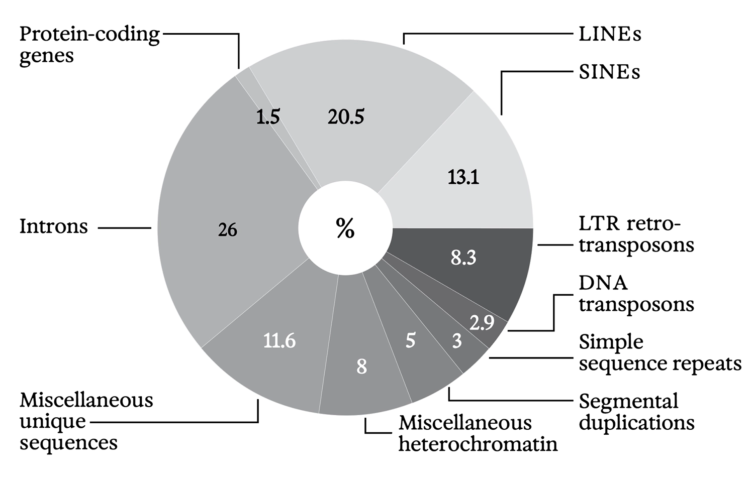
Relative proportions of the major families of human genomic elements, from Lander et al. 2001
The reproductive cycle of viruses is an often-told story. When traveling between cells, a virus looks like a bit of DNA or RNA packaged into a protein “envelope” capable of binding to a target cell and injecting its genetic payload. Once inside the cell, the viral code hijacks cellular resources to begin replicating, both copying its genetic material and manufacturing its envelope proteins. These assemble into more viruses. Maniacally cranking out viral proteins, the cell may eventually burst, releasing a flood of virus particles to repeat the cycle.
“Retroviruses” like HIV (the Human Immunodeficiency Virus, which causes AIDS) include additional “reverse transcription” machinery for permanently incorporating their genetic material into the cell’s DNA. This makes them a lot harder for the host to clear. The key enzyme, “reverse transcriptase,” wasn’t characterized until 1970, 59 but Barbara McClintock (1902–1992), working at Cold Spring Harbor Lab on Long Island, had made an earlier discovery that turned out to be closely related.
_shown_in_her_laboratory_in_1947.webp)
Barbara McClintock, Department of Genetics, Carnegie Institution at Cold Spring Harbor, New York, 1947
While studying the genetics of maize plants in the late 1940s and early ’50s, McClintock found mobile segments of DNA that seemed to be able to cut and paste themselves into different locations on the genome, producing differently mottled color patterns in corn kernels. 60 Although many of her colleagues were initially skeptical about these “transposons” or “jumping genes,” McClintock eventually won the Nobel Prize for her work.
A much wider zoo of “transposable elements” has since been discovered, some of which don’t just “cut and paste,” but “copy and paste” themselves; they are, in effect, replicators within our DNA. In fact, some of them are fully fledged retroviruses, including instructions not only for splicing their code into a host cell’s genome, but also for manufacturing envelope proteins, allowing that code to venture out into the world in search of other cells to infect.
Retroviruses are unsettlingly … intimate. HIV specifically targets immune cells, but if a retrovirus infects an egg or sperm cell, it can insert its code into an organism’s germ line, becoming a permanent part not only of that cell, but of an entire species. In a 2006 publication in the prestigious journal Nature, researchers at the University of Queensland in Australia reported catching a retrovirus in this act of becoming “endogenous” for the first time. 61 An epidemic of leukemia in koalas had first been traced to a retrovirus, then this retrovirus was found to have invaded the koala germ line over the previous century, causing the disease to become heritable.
Does this mean the end of koalas? Probably not.
The human genome is rife with signs that the same process has taken place many times in the history of our own species. At least eight percent of our genome consists of endogenized retroviruses, the remnants of such retroviral invasions. 62 Remember, eight percent is several times more DNA than codes for our “own” genes!
We usually think of viruses as mere disease agents, opportunistically parasitizing our cells to reproduce, since they have no reproductive machinery of their own. The reality may be very different, though. As many of us know from our recent experience with COVID, 63 viruses (and pathogens in general) tend to evolve into forms less lethal to their hosts over time, for obvious reasons—a dead host is a dead end for the pathogen, too. There’s mounting evidence that the relationship between virus and host can go even further, to become symbiotic. Retroviral code in our genome, for instance, has become fundamental to the formation of the placenta, the immune system, cell differentiation, and brain function. 64
Moreover, endogenous retroviruses are only the tip of an even larger iceberg. Nearly half of our genome consists of transposable elements of one kind or another. Some were probably once retroviruses, or vice versa. Fully sequenced genomes are often rife with lengthy stretches of highly repetitive sequences, from long and complex to mere alternations of two or three symbols—evidence of sub-replicators running amok.
Our genomes, in other words, are not only reproduced as a whole, but include working reproductive sub-sequences at many scales. Some are new and can still cause disease; others are older and may have lost the ability to make viral envelopes or the other machinery needed to become infectious; and yet others have integrated themselves so deeply into our own code that they are no longer distinct. Some of this code even serves critical functions in our bodies. It’s obvious that, at least by this last stage of the process, complete symbiosis has been established: neither the host nor the sub-replicator could survive, let alone reproduce, on its own.
In his 2009 book Virolution, 65 author and physician Frank Ryan goes further, arguing that viruses may have been symbionts all along. Plague viruses like HIV don’t come from nowhere; they are species jumpers. We know that HIV was originally SIV, the Simian Immunodeficiency Virus, variants of which are endemic to Old World primates including African green monkeys, sooty mangabeys, mandrills, and chimpanzees. Yet many of these viruses don’t sicken their original hosts. 66
We also know that if a virus finds itself inside an organism whose physiology is too different from that of its original host, it can’t gain purchase—a lucky thing for you, if you’ve ever swallowed a mouthful of seawater, which likely contained about a billion virus particles! (Most would have targeted single-celled marine life.) The greatest danger seems to come from viruses adapted to a different but closely related species. Perhaps, when it kills, such a virus is doing its job: wiping out rivals who have invaded the original host’s territory.
Viruses could, in other words, work like an out-of-body immune system. Within our bodies, our immune systems seek out and destroy cells that are recognized as “not-us.” Outside our bodies, “our” viruses could be similarly seeking out and destroying whole animals who are recognized as “not-us.” Once a virus becomes endemic to a new population, though—even if it initially kills many—it will differentiate, co-adapt, and perhaps eventually go native.
One could consider bacterial pathogens through a similar lens; hence the well-documented plagues of smallpox that European colonists brought to the Americas, decimating Native populations, and the virulent (though less deadly) syphilis epidemic believed to have been brought back to Europe by Columbus. 67 Unlike bacteria, though, retroviruses don’t just take up residence in our environment or in our bodies, but fuse into our very genomes, becoming inextricably part of us—especially when they alter the germ line.
By sheer volume, our DNA appears to be made primarily of the layered remnants of many such past fusions. It seems clear that transposable elements and “endogenous viral elements” or EVEs have done much more editing of our genome in recent evolutionary history than mutation has. 68 And they have been at this for a long, long time. Based on the best available evidence, viruses are at least as old as the Last Universal Common Ancestor, if not older. 69
This ongoing ecology of mobile, self-reproducing, and even infectious genes causes the supposed “tree of life” to continue entangling with itself in the oddest ways. Fully a quarter of the cow genome, for instance, consists of copies of the retrotransposon BovB. BovB appears to have leapt many times between species to create a phylogenetic tree of its own, a “bizarre parallel universe where cows are more closely related to snakes than to elephants, and where one gecko is more closely related to horses than to other lizards.” 70 These are instances of “horizontal gene transfer” (HGT), long associated with bacteria, but clearly more universal. 71
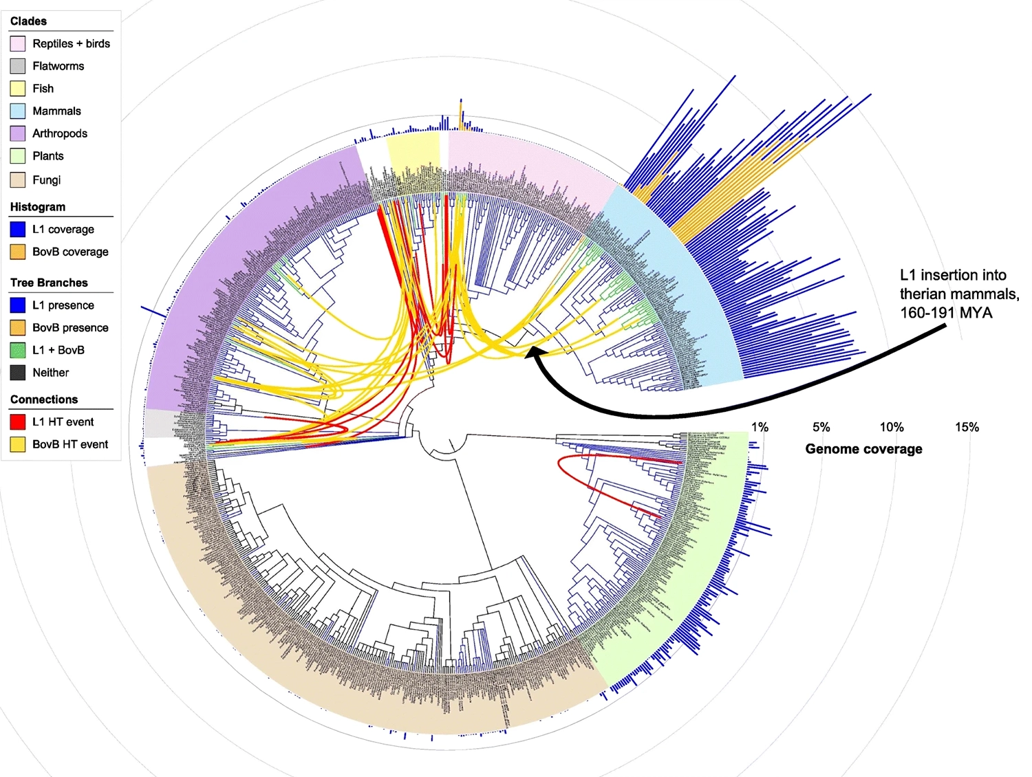
Map of the spread of the BovB and L1 retrotransposons across 759 species of eukaryotes, from Ivancevic et al. 2018
Whether a bit of new DNA is acting in the moment as friend, foe, or somewhere in between is just a matter of where on the symbiotic trajectory it falls. When brand new, it’s unlikely to be friendly. But if it has persisted for a long time, and especially if it has become endogenous, its dynamic stability implies that it will have become non-lethal or even friendly due to combined evolutionary pressures on host, invader, and “host plus invader” as a “holobiont” or symbiotically fused entity. If some gene or other functionality in the fused code proves valuable to the larger whole, that functionality will be conserved, even as the sub-replicator’s reproductive capability degrades and eventually vanishes. Perhaps that is how new genetic functionality arises in general.
In this light, random point mutation can even be seen as something like a minimal abiogenesis event, creating a tiny parasitic “life form” within the genome. On its own, it would of course be unable to reproduce, since it possesses no independent reproductive machinery; 72 then again, neither does a virus. So, like a virus, a mutation can reproduce—using the host’s resources, which will copy it along with everything else. When introduced into the genome of a sophisticated existing organism, such a tiny, random entity is unlikely to be friendly, though. As with any larger invasion, the mutation will either damage or kill its host (and itself, in the bargain) or achieve dynamic stability, either by being neutral or (occasionally) helpful.
Hence, just as replicator thermodynamics encompasses classical thermodynamics as a special case, evolution via symbiogenesis can encompass classical Darwinian theory as a special case. Point mutation is unlikely to be the main driver of evolution once life has taken off because it’s so much weaker and slower on its own than higher-order symbiogenesis. Unlike point mutation, a chunk of code that has already circulated, jumping around in the genome or even between species, isn’t random. It necessarily includes real functionality. And at least in some settings, that functionality has been under evolutionary pressure to help, or at least not kill, its host. Evolution picks up steam over time, with major evolutionary transitions becoming more frequent precisely because increasingly high orders of symbiogenesis become possible.
Compression
When code evolves through symbiogenesis, it will develop a curious statistical structure: parts of it will be copies (or near-copies) of other parts, and as those parts establish symbiosis, they’ll form a larger aggregate which will also copy itself as a unit. This is reminiscent of (though not the same as) a “fractal”: a structure that resembles itself at a cascade of ever-finer scales. Let’s take a short detour through fractals and their relationship to biology so that we can then consider the implications of evolution itself exhibiting certain fractal-like properties.
French-American mathematician Benoit Mandelbrot (1924–2010) is the figure most associated with fractals, though they were first described by English meteorologist Lewis Fry Richardson (1881–1953). In the aftermath of World War II, Richardson, a Quaker, had been trying to build a mathematical model to predict the likelihood of conflicts between countries. One of the parameters in his model was the length of their common border. He was perplexed to find, though, that certain borders didn’t appear to have agreed-upon lengths. The Portuguese, for instance, reported that their border with Spain was 613 miles long, but the Spanish claimed that it was 754 miles long. This seemed like a weirdly large discrepancy for what ought to have been an easily surveyed distance!
Richardson eventually figured out what was going on: the Spanish were using a higher-resolution map. Every twist and turn the Portuguese could see in the Minho, Douro, and Guadiana rivers separating the countries had finer-scale twists and turns only visible on the Spanish map. Richardson showed that, if zooming in on any given meandering revealed more meanderings, the total length of a “self-similar” curve like a coastline or a river can grow without limit as one measures it with an ever-smaller ruler. 73
The coast of Britain measured with rulers of different lengths
“Fractal geometry” is thus very different from the Euclidean geometry we all learned in school, where the length of a line or curve is well-defined and doesn’t blow up when you zoom in. Of course, in real life, one can’t zoom in forever, but fractals are still important mathematical tools for understanding structures that are self-similar over a range of scales, like rivers and coastlines.
Living organisms exhibit obvious fractal properties in certain of their structures, such as tree branches, bronchial tubes, and circulatory systems. In structures like these, fractal geometry over some range of scales offers an elegant design solution to a biophysical problem. For instance, blood carrying oxygen and nutrients needs to reach every cell in the body, which means that oxygenated blood has to be pumped through a branching network of tubes, and these tubes—which are, in Euclidean terms, one-dimensional—have to repeatedly subdivide to “fill” three-dimensional space. Hence, we have fractally branching (and then merging) networks of arteries, arterioles, capillaries, venules, and veins.
By working out the design properties of such fractal networks and their implications, theoretical physicist Geoffrey West and his collaborators at the Santa Fe Institute have figured out many fundamental “scaling laws” in biology. 74 One of the most well-known results from this body of work explains why every mammalian heart will beat about 1.5−2 billion times over a lifetime, whether it belongs to an Etruscan shrew (weighing a twentieth of an ounce, and living a year or so), or a blue whale (weighing over three hundred thousand pounds, and living about a century).
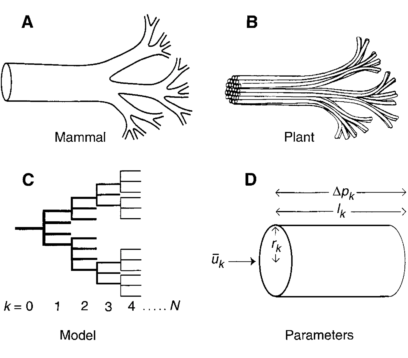
Fractal branching in mammalian circulatory systems and plants, from West, Brown, and Enquist 1997
Self-similarity in general yields “power law” scaling relationships, which look like straight lines when plotted on logarithmic axes. 75 Body mass, for instance, has power-law relationships with metabolic rate, the total length of the circulatory system, and lifespan. 76 Combining various power-law relationships to calculate the number of heartbeats in a lifetime causes all the scaling variables to cancel out beautifully, yielding the famous 1.5−2 billion beat constant. While the theory is not exact (humans, for example, live somewhat longer than predicted), it does a remarkable job of parsimoniously explaining a wide range of phenomena.
Is life in general a kind of fractal, then? No. A rhyme by British mathematician Augustus De Morgan is often invoked in describing fractals:
Great fleas have little fleas upon their backs to bite ’em,
And little fleas have lesser fleas, and so ad infinitum. 77
The poem is funny precisely because it is absurd: unlike an idealized fractal coastline, living systems are, in general, profoundly dissimilar across scales. 78 While there are rare instances of the kind De Morgan describes—such as hyperparasitoid wasps, tiny parasites that lay their eggs inside bigger wasps—one does not generally zoom in on a flea to discover a smaller flea, let alone ad infinitum.
Two further levels of fractal elaboration on Mandelbrot’s N=5, N=6, N=7 and N=8 coastline patterns
Indeed, even coastlines are best characterized, in real life, as “multifractals”: systems with repetitive structure at every scale, but variability across scales. 79 As a result, their power laws may also vary. For instance, zooming in twofold at one level of magnification, where the ruggedness is especially pronounced, might cause the apparent length to scale up by 21.5≈2.83, while zooming in twofold at a magnification where the coastline appears smoother might only cause the apparent length to scale up by 21.16≈2.24. Every bump has bumps on it, but the bumps at one scale are shaped differently from the bumps at another. 80
Similarly, although genomes are always replicated, and are made of other genomes that are themselves replicated, every whole is different from its parts, just as an integrated circuit is different from a transistor. How, then, would one go about quantifying this multifractal-like property in a genome?
The answer is closely related to data compression. Consider bff. In its initial state, the tapes consist of random bytes; there’s no repetitive structure. If we were reading through the tapes one byte at a time, the next byte would have an equal probability of assuming any value, from 0 to 255, independent of any of the previous bytes. Therefore, the sequence is entirely unpredictable, which means that if you were to try compressing the soup with file compression software, like ZIP, the compressor wouldn’t be able to squeeze the file size at all. (This is, harkening back to thermodynamics, a working definition of a completely disordered state.)
Data are redundant—that is, compressible—precisely to the degree that they are predictable, or, equivalently, exhibit order. Compression algorithms like those in ZIP work by looking for patterns already encountered in the data stream and exploiting those patterns to encode subsequent data using as few bits as possible. The usual trick is to incrementally build a dictionary or “phrase book” out of the source material, and to substitute sections of the text for pointers into this dictionary whenever the pointer can be encoded in fewer bits than the original text. The dictionary is, in effect, a predictive model, and since the compressor builds that model incrementally as it compresses, the decompressor is able to incrementally reconstruct an identical copy of the model as it decompresses.
Absent any prior knowledge about how to model a long sequence, describing it in terms of previously encountered parts of itself is a good strategy. The full text of this book ZIPs down to about thirty-five percent of its original size as a raw text string—since some letters occur more often than others, many words repeat, and those words often combine into stock phrases. 81
When bff undergoes its sharp transition to whole-tape replication, the tapes suddenly become highly compressible; they squeeze down to just five percent of their original size. Interestingly, many regions of the human genome are highly compressible too. These data streams compress so well because, at any given point in the sequence, one can often make a pretty good guess as to what the next letter will be, simply by looking for the longest previous sequence that matches the current context.
Such matches arise due to replication. In the human genome, we’re not talking about replication at the level of the individual, but, rather, at the level of transposable elements (or their fossil remnants) within our genome. Similarly, even a single bff tape is highly compressible, because it formed through a symbiotic fusion of smaller replicators … and these replicators are themselves likely to be either copies of each other or related, having formed out of yet smaller imperfect replicators … which are themselves either copies or related.
Like fractals, sequences of symbols constructed by repeatedly copying sub-sequences of all lengths exhibit power-law scaling—in this case, between the lengths of repeated sequences and their frequency. For instance, a replicated sequence twice the length of another might be found half as often—which is pretty often! (These statistics would be dramatically different for random sequences, where increasing the sequence length would cause a much faster exponential decline in expected frequency. 82 ) Sequences constructed according to a fixed self-copying rule are, in a sense, infinitely compressible, for they contain only as much information as it would take to write down the recipe, no matter how long the sequence.
By contrast, in a complex replicating system like bff—let alone the genome—the way any particular set of replicating sub-sequences combine to form a larger replicating sequence will always be specific. It will depend on the functional particulars of how those parts come together to make a working whole. Therefore, each such combination adds novelty or information. However, that information will be much less than would be needed to specify an arbitrary symbol sequence of the same length.
When we look for this property in bff and in human genome data, that’s just what we find! Not only do both compress very well; they also compress better and better the longer the stream of data gets. For instance, a single bff tape compresses somewhat, but the whole soup compresses better, and as the size of the soup grows, the compression ratio continues to improve—though no matter how much has already been seen, the remainder is never fully predictable.
Similarly, while a single stretch of a human genome already compresses well, the whole genome compresses better. In the statistical context of many other human genomes, so much of the information in your genome is redundant that it could be compressed to a file size small enough to send as an email attachment. 83 The pattern continues if we zoom yet farther out to consider genomes across species. Hence the famous statistic that the human genome is ninety-eight percent identical to the chimpanzee genome … and sixty percent similar to that of the fruit fly!
While common ancestry alone can explain many of the similarities across species (though not all, as BovB illustrates), such classical Darwinian arguments can’t explain why the genome of a single individual is also so repetitive. That only makes sense when we begin to consider genomes to be made out of smaller genomes.
DNA and bff tapes, in other words, are both systems that evolve through what we could call “multifractal symbiosis.” Our genomes are aggregates of cooperating replicators, all the way down. That’s why they are so compressible. But it’s also why wonderful new kinds of complexity emerge at every scale—and therefore why, in biology, we can always learn something new by zooming in or out.
Embodiment
There is a profound yet subtle relationship between the multifractal properties of our bodies and the multifractal properties of the genome.
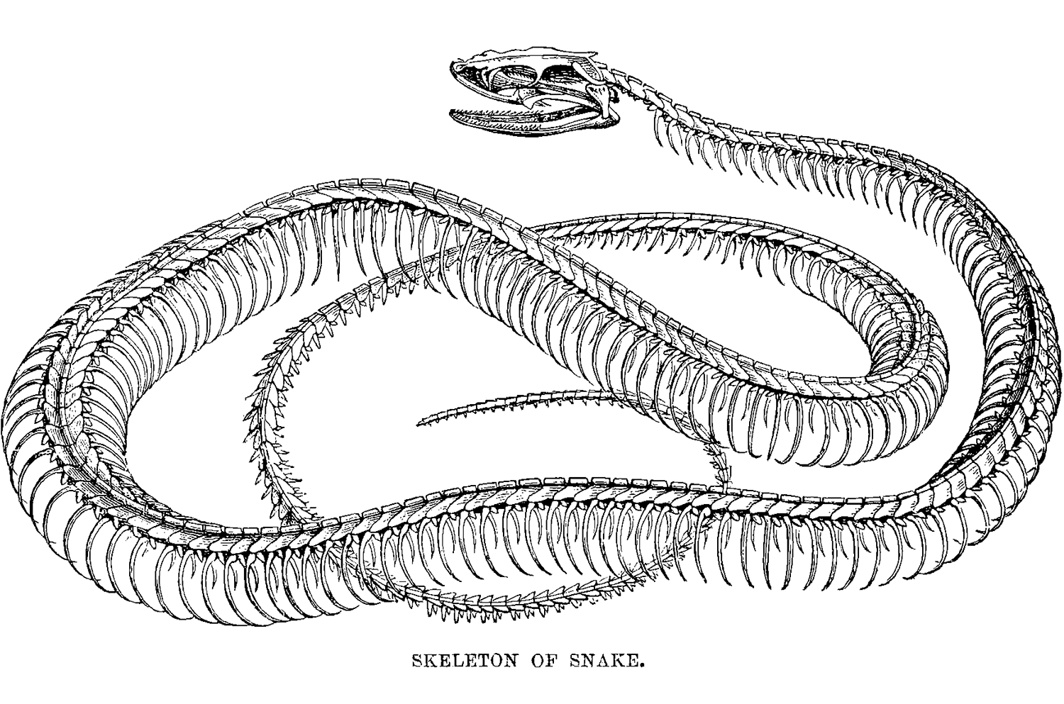
Snake skeleton from Lydekker, The Royal Natural History, 1893
The relationship is subtle because the genetic code is by no means a one-to-one blueprint explicitly representing the body’s final shape. One might imagine, for instance, that because a snake has hundreds of ribs, it might have a stretch of DNA coding for a vertebra and rib pair that might have replicated itself a few hundred times in the snake’s genome. Could snakes be the result of a retrotransposon coding for ribs run wild, like BovB?
Not exactly. So-called “Hox” genes, shared widely among animals, control overall body plan, and they “execute” their program using a combination of gene regulation and the kind of distributed computation Turing described in his work on morphogenesis. During embryonic development, ribs begin as a self-organized standing wave in the concentrations of chemical morphogens—the same kind of process that gives cows their spots and tigers their stripes. Whereas patterns in skin coloration merely involve varying pigmentation, though, the developmental program for a rib involves many subsequent morphogenetic steps.
This mechanism is vastly more powerful, general, and evolvable than merely replicating some “build a rib” code. It reuses code, just as any decent programmer would: invoking the same “build a rib” function a hundred times instead of copying and pasting it a hundred times. Thus, tweaking rib flexibility or curvature involves making one change, not a hundred.
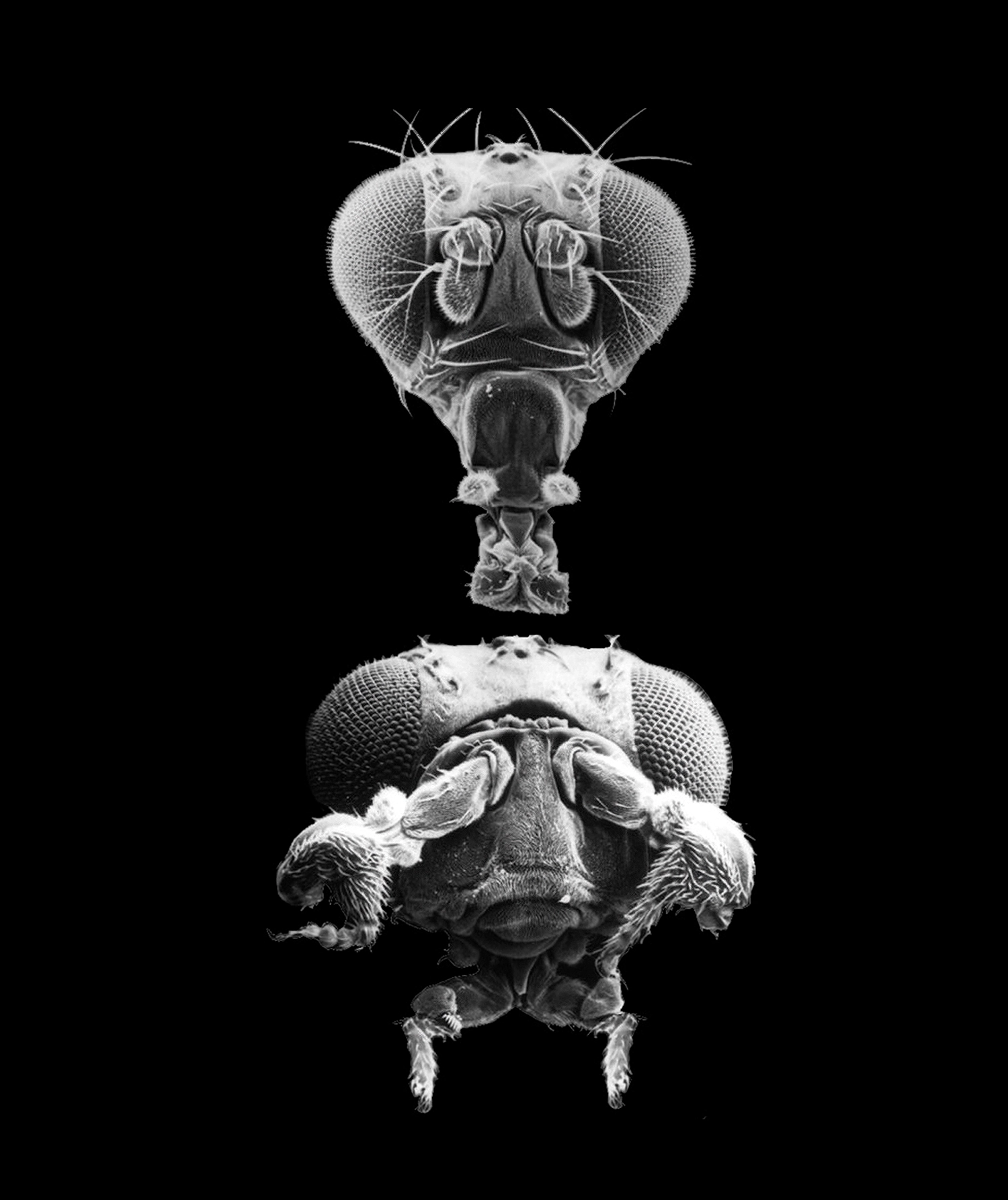
A mutation in the Antennapedia (or “Antp”) Hox gene of the fruit fly causes an extra pair of legs to grow out of the head in place of antennae, illustrating compositionality in body construction. Top: wildtype; Bottom: mutant.
Evolution can produce real programs that reuse code because life is computational. Remember that if you’re a replicator of the kind von Neumann described, you need to contain instructions for building yourself, including a machine B to copy those instructions, and a machine A, the “universal constructor,” to follow them. The universal constructor is the engine not only of reproduction, but also of growth, development, healing, and maintenance. It created your circulatory system and skin during embryonic development; it also heals your skin and replaces the torn capillaries underneath when you get a cut. As long as you are alive, your body will continuously construct and reconstruct itself. The code never stops running.
And since a universal constructor is a kind of Universal Turing Machine, its computations, or equivalently mathematical functions, are inherently “compositional”: complex functions (or programs) can be made of sub-functions, which can in turn be made of sub-sub functions … until, at bottom, everything could be expressed in terms of the elementary instructions of a Turing machine.
Functions can even be made out of themselves. In computer science, this is known as “recursion.” The Fibonacci sequence, for example—1, 1, 2, 3, 5, 8, 13, 21, and so on, where each number is the sum of the previous two—is most easily expressed as the recursive function f(n)=f(n−1)+f(n−2) for numbers greater than 1, with f(0)=f(1)=1. We find Fibonacci numbers in biology all the time, as in the spiral pattern of a pine cone, the head of a sunflower, and the chambers of a nautilus. This is a clue that recursive computation takes place in the construction of pine trees, sunflowers, and nautiluses. 84
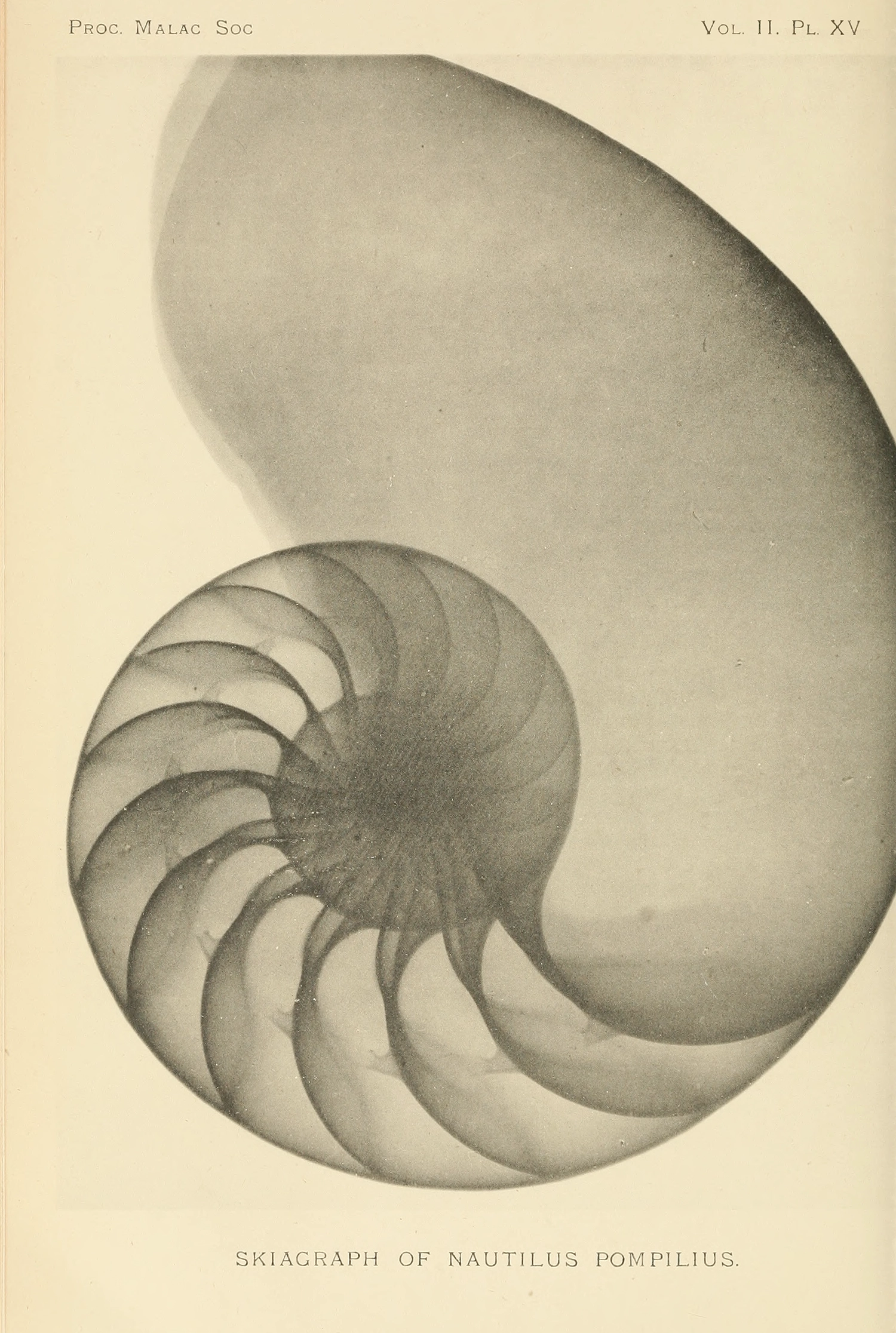
1896 skiagraph (x-ray photograph) of a Nautilus pompilius
The smoking gun, though, is the growth of self-similar structures in the body. Compositionality and recursion are what allow genetic code to build a many-tiered fractal like the circulatory system. Code for building ribs or nautilus segments could, in theory, just be copied a couple hundred times, but that’s not possible for arteries, veins, or capillaries, where the number of segments and branches becomes astronomically large. The blood vessel branching code must get reused. And with relatively minor tweaks, it must be possible for the parameters of that code to be adjusted so that the branching stops at the appropriate size for a shrew, or goes on to construct something the size of a blue whale, since shrews and whales are, in the grand scheme of things, close relatives.
From an evolutionary perspective, compositionality implies a hierarchical network of symbiotic relationships. The bacteria that became mitochondria and the archaea that engulfed them each started with the code they needed to reproduce themselves. When they merged into a eukaryote, they still needed to retain the instructions for their own reproduction, but they also needed to evolve additional functionality for mutual regulation. When eukaryotes became multicellular, the same process needed to happen again; our cells still know how to reproduce individually, and, indeed, cellular reproduction is a fundamental operation involved in the larger-scale growth and reproduction of a whole animal.
What is true of evolution is also true of an individual organism’s development. 85 Blood vessels, for instance, aren’t just Euclidean line segments, but tubes made of layers of smooth muscle cells. Each of those cells contains a complement of organelles, and each mitochondrion in each of those cells contains its own membranes and loop of bacterial DNA. A living organism is a compositional structure par excellence. It could only be built computationally, through the composition of many functions. And life could only have evolved as the hierarchical composition of those functions—that is, through symbiogenesis.
Daisyworld
All definitions of life are controversial, most seem to require caveats or exceptions, and none has advanced our understanding of biology. Frustrated with this state of affairs, biochemist Andrew Ellington has gone so far as to assert that “there is no such thing as life. Life is not a meaningful scientific term. It is a term for poets, not scientists.” 86
Ellington’s position may sound extreme, but it’s more defensible than the dogmatic definition in many biology textbooks: that living organisms have “the ability to eat, metabolize, excrete, breathe, move, grow, reproduce, and be responsive to external stimuli.” 87 By this definition, viruses aren’t alive, which might seem reasonable. But neither are mules or worker bees, since they are sterile!
Or consider a leaner definition popular among astrobiologists: “life is a self-sustaining chemical system capable of Darwinian evolution.” 88 Better, but by this definition, parasites are not alive, since they aren’t self-sustaining. Then again, is any life form truly self-sustaining? (Not if it eats.) How can a “self” be meaningfully circumscribed? And while life on Earth is based on chemistry, should we really insist on this as a requirement? Functionalism would argue otherwise.
So, here’s my own attempt:
Life is self-modifying computronium arising from selection for dynamic stability; it evolves through the symbiotic composition of simpler dynamically stable entities.
Notice that my definition doesn’t stipulate any specific function. However, in defining life computationally, it is functional. And in a world where the Second Law holds, dynamic stability implies that those functions must include some combination of self-construction, self-repair, or reproduction. All of these are computations that require code to be able to read and write code, hence the “self-modifying” qualifier.
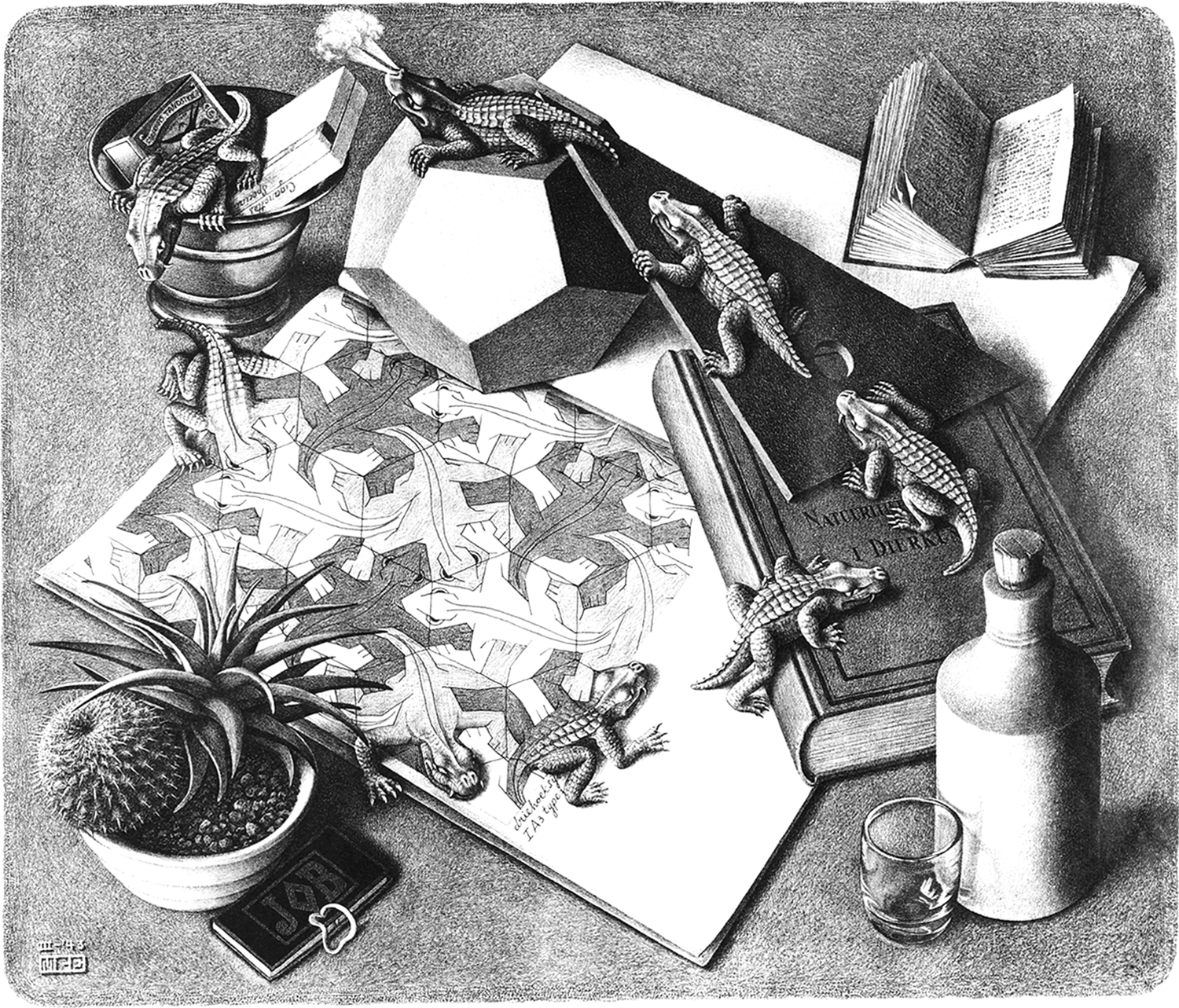
M. C. Escher, Reptiles, March 1943
“Computronium” is generally understood to be a phase of matter, but the “matter” here could be anything that can support computation, including bytes in bff or pixels in a cellular automaton. Furthermore, unlike gases, liquids, or solids, which are essentially uniform at macroscopic scales, the phase of matter associated with life is necessarily lumpy. One reason is that a uniform material can’t carry out general computation; computronium must, at its finest scale, contain distinct interacting components.
There’s a deeper reason, too. Dynamic stability implies the existence of discrete units—a self, or a population of selves—for without some model of a self or selves it would be impossible to say what is stable. And since life composes itself symbiotically, there are “whats” at multiple scales—in our case, from molecules to mitochondria, cells, whole organisms, and beyond. Studying each “what” requires zooming in or out to focus on the dynamic stability of a different kind of entity.
At the most zoomed-out scale, life consists of a single “lump”; for us, that would be the Earth. Is it, too, alive? Physicist and astrobiologist Sara Walker argues that it is not, precisely because it’s a singleton. Walker believes that the Earth will only become alive if and when we colonize another planet, thereby “reproducing.” 89 My definition of life doesn’t require reproduction, but it does require dynamic stability; can that even be defined for a singleton?
It can, in a sense first formalized in the 1970s and ’80s by the independent scientist James Lovelock, together with Lynn Margulis and others. Their “Gaia hypothesis,” named after the Greek Earth-goddess, is based on the observation that our planet as a whole is homeostatic. Negative feedback loops actively maintain various biosphere parameters within ranges friendly to life (though many mechanisms, like the one regulating the sea’s salinity, are still poorly understood). Earth’s temperature, for instance, has oscillated within a relatively narrow band for hundreds of millions of years, even though the Sun has grown hotter over time. Earth’s temperature remains stable enough for life because it actively warms and cools itself, and it warms and cools itself because it is alive.
The mechanism whereby such self-regulation arises is no mystery, and indeed boils down to Darwinian selection for dynamic stability. A simulation of a highly simplified Earth-like planet Lovelock called “Daisyworld” illustrates how this works. 90 Daisyworld has only two species: black daisies and white daisies, both of which have reproductive rates that depend on temperature—a sweet spot at a balmy 72.5°F, declining gradually to zero if the heat is below 41°F or above 104°F. Black daisies warm the planetary surface by absorbing sunlight, while white daisies cool it by reflecting sunlight. Careful mathematical analysis shows that black and white daisy populations will dynamically adjust to regulate the mean surface temperature, keeping it close to the sweet spot over a factor of two in solar luminosity—a remarkable range, which, on a lifeless planet, would yield temperatures ranging from 32°F–140°F.
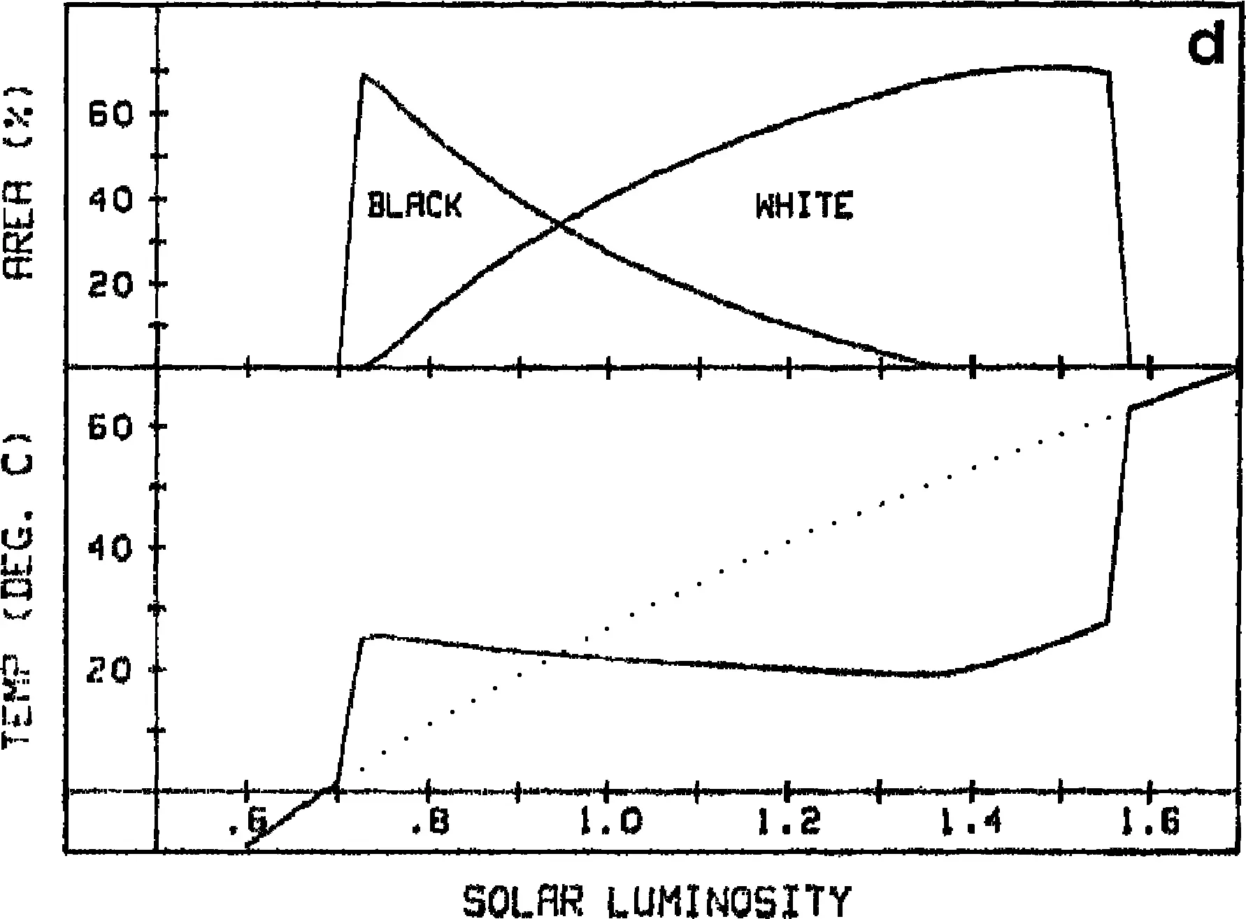
Black and white daisy populations work in tandem to stabilize temperature on Daisyworld over a factor of two in solar luminosity; A. J. Watson and Lovelock 1983.
While the detailed analysis is complicated, even for a simple two-species ecology, the mechanism behind this homeostatic tendency is generic. Roughly speaking, it holds whenever there exist species whose populations both depend on the environment and have an effect on that environment. Some homeostasis occurs even with just a single species (in Daisyworld, either black or white daisies), but homeostasis is more robust with multiple species that can, like opposable muscles, perturb the environment in one direction or another.
So, in my view, a planet like Daisyworld or Earth is indeed alive, for it not only contains computational life forms (and therefore does a lot of computation in the aggregate), but it also self-modifies to achieve dynamic stability. Daisyworld shows, in other words, how evolution can still operate with a population size of one. The key is modularity: its parts are also alive, and can themselves undergo evolutionary selection.
Aspen forests offer a useful parallel. Aspen trees send out horizontal roots that can sprout a trunk and grow into another tree. Or is it another trunk of the same tree? “Pando,” in Sevier County, Utah, is a quaking aspen covering more than a hundred acres and estimated to weigh over thirteen million pounds. Although each of its forty-seven thousand or so trees (trunks? stems?) have finite lifespans, the whole forest can be understood as a single, immortal organism that—if it were confined to a fertile valley surrounded by impassable mountains—might never reproduce.
The Pando quaking aspen, Utah
Although an aspen forest’s genetics are locked in—since every apparent tree is a clone—Darwinian selection still takes place, in that trunks in favorable places will flourish and reproduce, while those in unfavorable places won’t. Individual trees can’t move, but the forest can—an example of an “emergent capability.” As the valley’s climate shifts, the whole forest then will go on the march, creeping up and down the mountainsides to maintain homeostasis. It is thus entirely reasonable to call both the trees and the forest alive, just as it’s reasonable to call both you and your individual cells alive. So, too, the Earth as a whole.
However, this doesn’t imply that the Earth is “smarter than” the sum of its parts, or that it is conscious, just because we individually are, and we are part of it. In fact the social intelligence hypothesis, which we’ll explore in chapter 5, suggests that our consciousness arose as a result of social interaction. Our planet has no other living planets to socialize with. 91
The Earth is intelligent only to the degree that the models implicit in its feedback loops have kept it alive under gradually changing conditions for billions of years—a slow, vegetative kind of intelligence with limited predictive power. Although now techno-humanity is starting to model both the Earth and the heavens, keeping telescopic “eyes” open for stray asteroids and radio “ears” cocked for alien transmissions. No dice … yet. But arguably our planet is rapidly becoming more intelligent and animal-ish, able to sense remotely and make long-range predictions, poised to respond proactively to threats and opportunities, should they arise—and assuming we can get our act together and re-establish a planetary homeostasis that includes humanity and technology.
Élan Vital
If life is computational, then are human-engineered (that is, “artificial”) computers alive? They are certainly purposive, or we couldn’t talk about them being broken or buggy. But hardware and software are, in general, unable to reproduce, grow, heal, or evolve on their own, because engineers learned long ago that self-modifying code (like bff, or DNA) is hard to understand and debug. 92 Thus, phones don’t make baby phones, or (alas) heal from their frequent injuries. Apps don’t write new versions of themselves.
And yet: there are more phones in the world this year than last year, and their cracked screens do often get repaired; apps acquire new features, become obsolete, and eventually reach end-of-life, replaced by new ones; and AI models improve from month to month. Electronic components and computer code also exhibit the same kind of compositionality we’ve seen in bff and DNA. It certainly looks as if technology is reproducing and evolving! 93 Debating its aliveness is thus a bit like the debate over whether viruses or parasites are alive.
Excerpt from Le Royaume des fées by Georges Méliès, 1903
If we zoom back out, putting technology and humans in the frame together, we can see that this larger, symbiotic “us” is certainly reproducing, growing, and evolving. 94 The emergence of technology, and the mutually beneficial—if sometimes fraught—relationship between people and tech is nothing more or less than our own most recent major evolutionary transition. Technology, then, is not distinct from nature or biology, but merely its most recent evolutionary development.
And what about that age-old inanimate stuff—rocks and rivers, mountains and beaches, clouds and storms? Water molecules in themselves are clearly not capable of general computation. Yet in the context of the hydrologic cycle, clouds, rainstorms, and rivers certainly serve critical ecological functions, and are profoundly shaped by life. Likewise, our planet’s metal and sand are shaped into steam engines and computer chips, just as calcium we ingest turns into bones and ionic currents. All of these materials and structures comprise parts of a grand network of Gaian interdependency. Why do we draw boundaries around certain networks of functions and insist that they are “alive,” while asserting the surrounding functions are not?
This way lies vitalism, a view espoused in various forms by a long line of philosophers from Posidonius of Apameia (circa 135–51 BCE, and undoubtedly reflecting a much older tradition) to Henri Bergson (1859–1941). Some modern thinkers, too, defend the vitalist position, such as Jane Bennett:
The quarantines of matter and life encourage us to ignore the vitality of matter and the lively powers of material formations […]. By vitality I mean the capacity of things—edibles, commodities, storms, metals—not only to impede or block the will and designs of humans but also to act as quasi agents or forces with trajectories […] or tendencies of their own. [… Our] analyses of political events might change if we gave the force of things more due. 95
We resist such ideas because we tend to reserve the notion of agency only for ourselves. The idea of agency in a molecule or a storm, let alone an abstraction like money, seems especially far-fetched. We also tend to think in terms of a hierarchy in which “we” (for whatever value of “we”) are at the top, and agency must surely diminish for anything “lower”—a view reminiscent of the medieval Great Chain of Being. 96 When we (hesitantly) extend “agency” to the nonhuman, we tend to do so only for things that act obviously, individually, and on fast timescales, rather than in the aggregate and on slower, more evolutionary ones. It might be time to re-examine these ideas more holistically.
My purpose here is not to follow in Bennett’s footsteps—though I do find her project worth taking seriously. Language is, necessarily, imprecise, no matter what definitions we pick. 97 This doesn’t mean that words are useless, though. When our language can become more rigorous and scientifically grounded, and when we use it to describe consistent patterns uniting a wide range of observations, we can start to see through ideological thickets.
I hope I have explained both clearly and rigorously how the phenomena that give rise to the complexifying dynamics of life apply much more broadly than to the entities we normally think of as “alive” or “agential.” Accordingly, we could expand our definitions of these existing words, or adopt new ones, or do a bit of each. Personally, I would find some broadening of the old everyday words helpful.
That would hardly break new ground. Many traditional, nominally “prescientific” worldviews embrace notions of aliveness, agency, and even personhood that are far broader than the modern Western ones. This seems a likely case of convergent evolution in languages and ideas, motivated by the common need among traditional societies to take symbiosis seriously to secure their own survival, and to flourish. Taking a broader view is practical as much as it is spiritual: encouraging richer modeling of agency in “nature” enhances a society’s dynamic stability, since all things in “nature,” ourselves included, are so mutually interdependent.
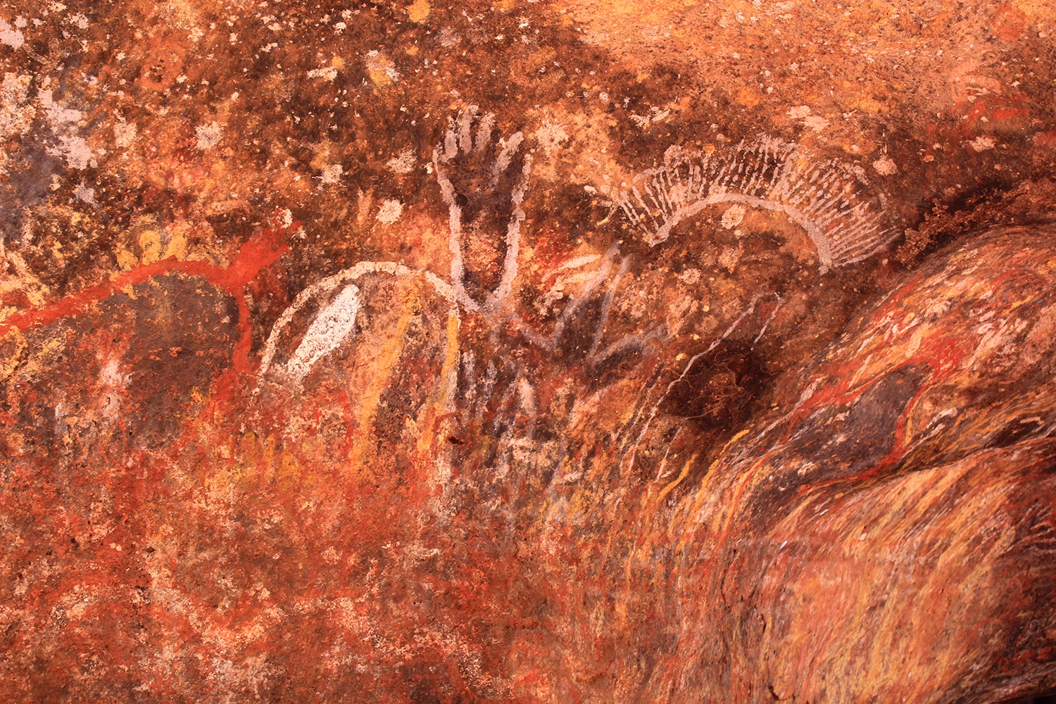
Aṉaŋu rock art, Uluṟu-Kata Tjuṯa National Park, Australia
Thus it can be useful to take the view of an animal, plant, or river at times, even if they can’t take ours, the better to care for them—and for ourselves. The same goes for the Earth as a whole. That, ultimately, is the best reason to consider adopting, or at least adapting, a more inclusive view of the animate. Potawatomi writer and biologist Robin Wall Kimmerer makes this case eloquently in her book Braiding Sweetgrass. 98
In agreeing with Kimmerer, I am not encouraging superstition. When scientists castigate animist beliefs as superstitious, they typically appeal to the materialist discoveries of the Enlightenment, which show that the atoms that make up our bodies are no different from the atoms that make up rocks or air. This is true. Atoms are atoms; they all obey the same rules. Hence, the Enlightenment model of a clockwork universe, governed by dynamical laws.
Yet as Schrödinger pointed out in 1944, our understanding of these laws—which he played such a central role in developing—remains incomplete. The laws as they stand do not account for the computationally complex, dynamically stable, symbiotic phenomena that comprise so much of our experience on Earth—indeed, without which there would be no such thing as experience at all. There would be no life, or purpose, or minds, or agency.
As we both embrace scientific rigor and start to figure out those “‘other laws of physics’ hitherto unknown,” 99 we should perhaps be less surprised to find the shoe on the other foot. What the poet Dylan Thomas called “the force that through the green fuse drives the flower” 100 drives all atoms, not just the ones we presume to be alive.

Detail of painting by Yalti Napangati depicting Marrapinti, Western Desert, Australia
W. Thomson 1871 ↩.
Peretó, Bada, and Lazcano 2009 ↩.
Robertson and Joyce 2012 ↩.
Remember, from chemistry class, that since hydrogen (H) consists of a single proton bound to a single electron, a positively charged hydrogen ion with its electron stripped off (H+) is just a proton. When proton concentration varies over space, the ensuing flow of ions generates an electric current.
Krebs and Johnson 1937 ↩. Krebs won the Nobel Prize in Medicine for this work in 1953.
M. C. Evans, Buchanan, and Arnon 1966 ↩.
Buchanan and Arnon 1990 ↩.
Today, a great majority of the organic fuel consumed by respiration in animals and fungi comes from plants, which fix carbon using photosynthesis instead of the more ancient reverse Krebs cycle.
Szathmáry and Smith 1995 ↩. The somewhat narrower term “evolutionary transitions in individuality” (ETI) is also increasingly used; Michod 2000 ↩.
Sagan 1967 ↩.
Woese 2002 ↩. In this book, I’ll use the terms symbiosis and symbiogenesis in broader ways than most biologists do, to include cooperation and eventual interdependence among entities of all kinds—in the spirit of molecular biologists who have framed the origins of life as symbiosis among “molecules in mutualism,” per Lanier, Petrov, and Williams 2017 ↩. See also Mizuuchi, Furubayashi, and Ichihashi 2022 ↩.
Konstantinidis, Ramette, and Tiedje 2006; Murray, Gao, and Wu 2021 ↩, ↩.
Raup and Gould 1974 ↩.
In some cases, like the car versus the horse and buggy, or photosynthesis versus the reverse Krebs cycle, a new technology crowds out an old one due to greater efficiency; however, even here, the crowding-out is often not total. There are still a few horses and buggies, and a few organisms using the reverse Krebs cycle.
Turing 1937 ↩.
Technically, a Turing Machine, whether universal or not, must always be able to increase its tape size if needed, while real computers have fixed storage limits—but for most purposes, close enough.
von Neumann 1945 ↩.
Both died young, Turing in 1954, at age forty-one, and von Neumann in 1957, aged fifty-three.
Turing 1952 ↩.
Many years later, German molecular biologist Christiane Nüsslein-Volhard identified the first real-life morphogen, the “Bicoid” protein, which forms a gradient along the fruit fly embryo to establish its segmented body plan. She won the Nobel Prize for this discovery, alongside Eric Wieschaus and Edward Lewis, in 1995.
von Neumann and Burks 1966 ↩.
In a more abstract form, mathematician Stephen Kleene had proven this result years earlier, a result known today as Kleene’s Second Recursion Theorem; Kleene 1938 ↩.
I’m using the term complex here in a colloquial sense; according to at least one technical definition (Kolmogorov complexity), if the instructions within the “simple” entity fully describe how to make the “more complex” one, they are actually of equal complexity.
J. D. Watson and Crick 1953 ↩.
While reversible computing is known to be theoretically possible, and has attracted some renewed interest in recent years because of its relevance to quantum computing, it remains largely unexplored.
Turing 2000 [1951] ↩.
Turing 1948 ↩. Infants’ brains are of course not random. Turing was right to believe, though, that randomness plays a major role in their initial “wiring”; subsequent learning and development strengthens some connections, while pruning many others.
Pesavento 1995 ↩.
Mordvintsev et al. 2020 ↩.
Agüera y Arcas et al. 2024 ↩. This work draws inspiration from classic work in ALife, especially Barricelli 1957; Fontana 1990; Ray 1991; Adami and Brown 1994 ↩, ↩, ↩, ↩.
Decrementing 0 wraps around to 255, the largest possible value for a byte, and incrementing 255 wraps around to 0.
You might have noticed that the original Brainfuck had eight instructions, including “
.” for “print” and “,” for “input.” Bff uses only “,” because instead of reading and writing to an external terminal or console, the tape reads and writes to itself. Thus copying a byte from one location to another requires only a single instruction. In our first paper describing bff, we included instructions “{” and “}” for moving the console pointer, but a stripped-down alternative, used here, simply initializes the data and console pointers with the first two bytes on the tape.Fontana 1990 ↩.
Amato 1991 ↩.
Schrödinger 1944 ↩.
The “very nearly” qualifier arises from the deep mathematical structure of relativistic quantum mechanics. A number of near-symmetries in physics, such as between positive or negative charge, left- or right-handedness, and time reversal, are not quite exact in quantum field theory, though according to the CPT theorem—the letters stand for charge, parity, time—reversing all three at once does yield an exact symmetry.
For the moment, I’m sidestepping a direct definition of the term disorder and its apparent subjectivity (is my desk disorderly or does it reflect an order only I can see?), but we will soon return to the central role of a model in distinguishing order from disorder; this is the link connecting thermodynamics to information theory.
The development of clocks and other complex machines in the Middle Ages set the scene, per Prigogine and Stengers 1984 ↩: “The clock world is a metaphor suggestive of God the Watchmaker, the rational master of a robot-like nature.” Newtonian dynamics reinforced the idea that the universe’s dynamics were deterministic and knowable, hence “robot-like.”
For now, I’ll use the term “Industrial Revolution” to refer to the first Industrial Revolution, the harnessing of fossil fuels beginning around 1800. Subsequent revolutions associated with electrification (around 1900), computerization (around 1980), and AI (around 2020) will be taken up in “Vulnerability,” chapter 10.
Smil 2008 ↩.
Agüera y Arcas 2023 ↩.
PV=nRT, where P is pressure, V is volume, T is temperature, n is the number of gas molecules or billiard balls, and R is the “ideal gas constant.”
Kinetic energy is proportional to the mass and squared velocity of the molecules.
More precisely, these are repulsive interactions between the electron orbitals of the molecules.
W. Thomson 1857 ↩.
Pross 2012 ↩.
Taleb 2014 ↩.
This is beautifully illustrated by a 2024 “RNA world” experiment in which, under lab conditions, a mutating, imperfectly replicating RNA molecule evolves into multiple forms that can persist indefinitely; Papastavrou, Horning, and Joyce 2024 ↩.
In the language of dynamical systems theory, thermodynamic stability is a fixed point, while DKS is a limit cycle.
Dawkins 1986 ↩.
Kauffman 1971 ↩.
In classical mythology, chimeras are “unnatural” combinations of animals—for instance, a fusion of lion, goat, and snake. As we’ll see, they aren’t so unnatural after all.
Yinusa and Nehaniv 2011 ↩.
This is not an absolute rule, since new parts can also evolve within an existing whole.
Lander et al. 2001 ↩.
Baltimore 1970 ↩.
McClintock 1950 ↩.
Tarlinton, Meers, and Young 2006 ↩.
She et al. 2022 ↩.
Horita and Fukumoto 2023 ↩.
Chuong 2018; Bakoulis et al. 2022; Russ and Iordanskiy 2023 ↩, ↩, ↩. Knocking out the “Arc” retrotransposon, likely of viral origin, renders lab mice unable to form new long-term memories, per Pastuzyn et al. 2018 ↩.
Ryan 2009 ↩.
Sharp and Hahn 2011 ↩.
Nasir and Caetano-Anollés 2015 ↩.
Yong 2013 ↩.
Unlike eukaryotes, prokaryotes (bacteria and archaea) have very low proportions of “junk DNA.” This is because copying and expressing DNA are energetically expensive, and prokaryotes are energy-constrained, limiting their maximum DNA length and imposing strong evolutionary pressure to rid themselves of code that can’t pull its own weight. However, a prokaryote’s “core genome” is typically only 60–70 percent of the total, with the remainder varying widely among strains. (Hence two E. coli bacteria can be as different from each other as a human and a fruit fly!) Horizontal gene transfer via transposons, viruses, or “plasmids” (exchangeable DNA loops) enables widespread copying of code snippets among bacteria, resulting in a complex tangle of reproducing bits of code conceptually similar to that described here for eukaryotes.
Though earlier, we similarly considered individual bff instructions as minimal or “atomic” replicating entities.
Mandelbrot rediscovered and generalized these findings in the 1960s; see Mandelbrot 1967 ↩.
West 2017 ↩.
For the mathematically inclined: power laws relating two variables x and y take the general form y=axb.
West, Brown, and Enquist 1997 ↩.
De Morgan and De Morgan 1872 ↩.
This makes sense, since the underlying processes that shape coastlines differ between scales of, say, a meter, versus a kilometer; see Mandelbrot 1989 ↩.
These particular numbers correspond to the smoothest, N=5, and roughest, N=8, of Mandelbrot’s coastline diagrams in his classic 1967 paper, “How Long Is the Coast of Britain?”
If I were a fancier writer and used fewer stock phrases, the book wouldn’t ZIP so efficiently. Using the same compression algorithm, James Joyce’s Ulysses can only be squeezed down to forty percent of its raw size!
In math: for a random string of symbols that can assume K values, a string of length L would occur with frequency f=K–L, while with replication occurring at all scales, string frequency scales like f~L–b.
Christley et al. 2009 ↩.
Recursion can’t be implemented by the ribosome on its own; I’ve used a bit of poetic license in identifying the ribosome with machine A. In reality, as morphogenesis illustrates, biological computation is more holistic and distributed. Like the “writing arm” of a von Neumann replicator, a ribosome is only one functional part of a larger, general-purpose biological machine A.
Carroll, Grenier, and Weatherbee 2013 ↩.
Ellington 2010 ↩.
Walker 2024 ↩.
Walker 2024 ↩.
Personal communication during the Antikythera Cognitive Infrastructures studio at Central Saint Martins in London, July 2024.
A. J. Watson and Lovelock 1983 ↩.
As will be discussed in “Crew of Eight,” chapter 5, the octopus may offer an example of a more modular route to high intelligence.
Computer viruses are a notable exception.
The case for technology being an evolutionary product of hierarchically composed functions is thoughtfully made, with many examples, by Arthur 2010 ↩.
As astronomer Robert Jastrow put it, “We are the reproductive organs of the computer” (Jastrow 1981 ↩); the same holds for technology in general. Samuel Butler made this case in a visionary 1863 essay entitled “Darwin Among the Machines,” a perspective revisited and updated at the end of the twentieth century by science historian George Dyson; Butler 1863; G. Dyson 1998 ↩, ↩.
J. Bennett 2010 ↩.
Lovejoy 1936 ↩.
Enfield 2024 ↩.
Kimmerer 2013 ↩.
Schrödinger 1944 ↩.
Thomas 1934 ↩.